Iterative forecasting
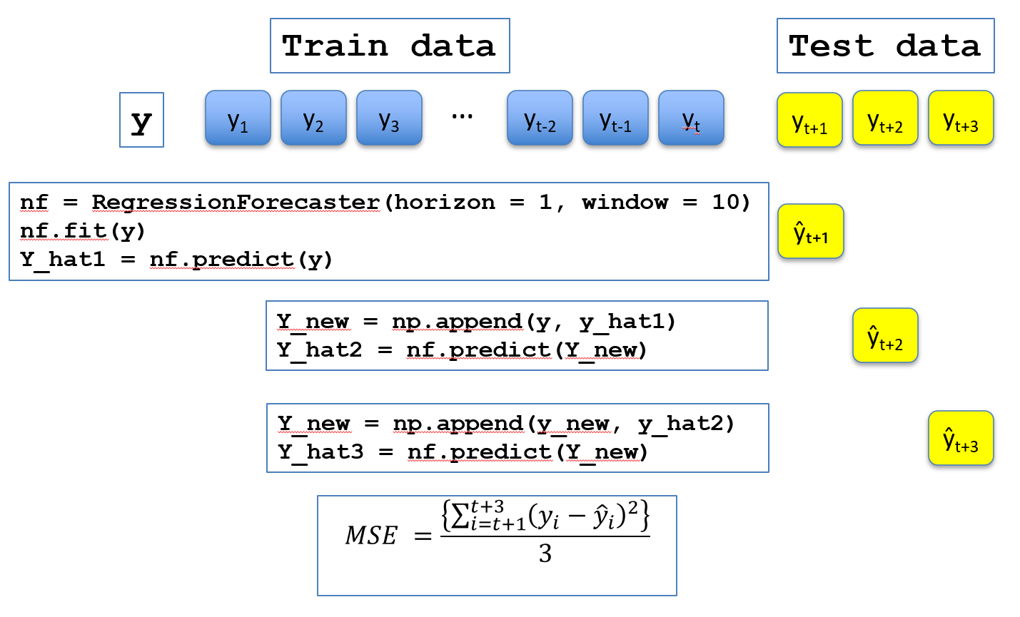
Iterative forecasting (sometimes called recursive) involves repeatedly predicting with a forecaster by adding predicted values to the actual values. Suppose you have a series of length \(n\) and you want to forecast the next 20 steps, the pseudocode for this is as follows.
call f.fit(y)
for i ← 1 to predictive_horizon do
    preds[i - 1] ← f.predict(y)
    y.append(preds[i - 1])
end for
In contrast to direct forecasting, the iterative forecast only ever fits a single model. You can visualise the process as follows
We will demonstrate direct forecasting with the airline data
[ ]:
from aeon.datasets import load_airline
from aeon.visualisation import plot_series

airline = load_airline()
_ = plot_series(airline)
[ ]:
import matplotlib.pyplot as plt
import numpy as np

y_train = airline[:100]
y_test = airline[100:120]
plt.plot(np.arange(0, len(y_train)), y_train, label="Train", color="blue")
plt.plot(
    np.arange(len(y_train), len(y_train) + len(y_test)),
    y_test,
    label="Test",
    color="orange",
)
plt.legend()
plt.xlabel("Time")
plt.ylabel("Value")
plt.title("Train/Test Split of Time Series")
plt.show()
We want to train a forecaster on the train set and forecast predictions for the subsequent test steps. The RegressionForecaster is a window based forecaster that by default uses linear regression to predict one step ahead. It requires a window parameter. See the forecasting with regression notebook for details. The forecast() method makes a single forecast horizon steps ahead.
[ ]:
from aeon.forecasting import RegressionForecaster

reg = RegressionForecaster(horizon=1, window=10)
p1 = reg.forecast(y_train)
print(" First forecast = ", p1)
what if we want to predict further ahead? The direct strategy, described here retrains the model for each set, changing the forecasting horizon. This can be computationally intensive. As an alternative, the iterative strategy uses the predicted value and predicts without refitting.
[ ]:
y_new = np.append(y_train, p1)
p2 = reg.predict(y_new)
y_new = np.append(y_new, p2)
p3 = reg.predict(y_new)
print(f" second forecast = {p2} third forecast = {p3}")
there is a function in the base class to make iterative forecasting easier.
[ ]:
y_hat = reg.iterative_forecast(y=y_train, prediction_horizon=20)

plt.plot(np.arange(0, len(y_train)), y_train, label="Train", color="blue")
plt.plot(
    np.arange(len(y_train), len(y_train) + len(y_test)),
    y_test,
    label="Actual",
    color="orange",
)
plt.plot(
    np.arange(len(y_train), len(y_train) + len(y_hat)),
    y_hat,
    label="Predicted",
    color="green",
    linestyle=":",
)
plt.legend()
plt.xlabel("Time")
plt.ylabel("Value")
plt.title("Train/Test/Pedicted")
plt.show()
Looking closer, we can see the errors our forecaster is making.
[ ]:
plt.plot(y_test, label="Actual", color="orange")
plt.plot(y_hat, label="Predicted iterative", color="green", linestyle=":")
plt.legend()
plt.xlabel("Time")
plt.ylabel("Value")
plt.title("Pedicted and Actual over the test interval")
plt.show()
It seems to be underestimating the peaks and troughs. Contrast this to the direct strategy which results in very different forecasts
[ ]:
y_hat2 = reg.direct_forecast(y=y_train, prediction_horizon=20)
plt.plot(y_hat2, label="Predicted direct", color="blue", linestyle=":")
plt.plot(y_test, label="Actual", color="orange")
plt.plot(y_hat, label="Predicted iterative", color="green", linestyle=":")
plt.show()
[ ]:
import matplotlib.pyplot as plt
import numpy as np
from statsmodels.tsa.exponential_smoothing.ets import ETSModel

from aeon.datasets import load_airline
from aeon.forecasting.stats import ETS

airline = load_airline()
y_train = airline[:100]
y_test = airline[100:120]

ets = ETS(
    error_type="additive",
    trend_type="additive",
    seasonality_type="additive",
    seasonal_period=12,
)
statsmodels_ets = ETSModel(
    endog=y_train,
    error="add",
    trend="add",
    seasonal="add",
    seasonal_periods=12,
    damped_trend=False,
)

ets_forecasts = ets.iterative_forecast(y_train, 20)
sm_model = statsmodels_ets.fit()
statsmodels_forecasts = sm_model.forecast(steps=20)
print(f"Alpha: {ets.alpha_}, Beta: {ets.beta_}, Gamma: {ets.gamma_}, Phi: {ets.phi_}")
print(
    f"Alpha: {sm_model.alpha}, Beta: {sm_model.beta if sm_model.has_trend else 'N/A'}, \
        Gamma: {sm_model.gamma if sm_model.has_seasonal else 'N/A'}, \
            Phi: {sm_model.phi if sm_model.damped_trend else 'N/A'}"
)
# plt.plot(np.arange(0, len(y_train)), y_train, label="Train", color="blue")
plt.plot(
    # np.arange(len(y_train), len(y_train) + len(y_test)),
    y_test,
    label="Actual",
    color="orange",
)
plt.plot(
    # np.arange(len(y_train), len(y_train) + len(ets_forecasts)),
    ets_forecasts,
    label="Aeon",
    color="red",
    linestyle=":",
)
plt.plot(
    # np.arange(len(y_train), len(y_train) + len(statsmodels_forecasts)),
    statsmodels_forecasts,
    label="Statsmodels",
    color="green",
    linestyle=":",
)
plt.legend()
plt.show()
[ ]:
[ ]:
Generated using nbsphinx. The Jupyter notebook can be found here.
![]()