Benchmarking time series regression models
Time series extrinsic regression, first properly defined in [1] then recently extended in [2], involves predicting a continuous target variable based on a time series. It differs from time series forecasting regression in that the target is not formed from a sliding window, but is some external variable.
This notebook shows you how to use aeon to get benchmarking datasets with aeon and how to compare results on these datasets with those published in [2].
Loading/Downloading data
aeon comes with two regression problems in the datasets module. You can load these with single problem loaders or the more general load_regression function.
[20]:
from aeon.datasets import load_cardano_sentiment, load_covid_3month, load_regression

trainX, trainy = load_covid_3month(split="train")
testX, testy = load_regression(split="test", name="Covid3Month")
X, y = load_cardano_sentiment()  # Combines train and test splits
print(trainX.shape, testX.shape, X.shape)
(140, 1, 84) (61, 1, 84) (107, 2, 24)
there are currently 63 problems in the TSER archive hosted on timeseriesclassification.com. These are listed in the file datasets.tser_datasets
[21]:
from aeon.datasets.tser_datasets import tser_soton

print(sorted(list(tser_soton)))
['AcousticContaminationMadrid', 'AluminiumConcentration', 'AppliancesEnergy', 'AustraliaRainfall', 'BIDMC32HR', 'BIDMC32RR', 'BIDMC32SpO2', 'BarCrawl6min', 'BeijingIntAirportPM25Quality', 'BeijingPM10Quality', 'BeijingPM25Quality', 'BenzeneConcentration', 'BinanceCoinSentiment', 'BitcoinSentiment', 'BoronConcentration', 'CalciumConcentration', 'CardanoSentiment', 'ChilledWaterPredictor', 'CopperConcentration', 'Covid19Andalusia', 'Covid3Month', 'DailyOilGasPrices', 'DailyTemperatureLatitude', 'DhakaHourlyAirQuality', 'ElectricMotorTemperature', 'ElectricityPredictor', 'EthereumSentiment', 'FloodModeling1', 'FloodModeling2', 'FloodModeling3', 'GasSensorArrayAcetone', 'GasSensorArrayEthanol', 'HotwaterPredictor', 'HouseholdPowerConsumption1', 'HouseholdPowerConsumption2', 'IEEEPPG', 'IronConcentration', 'LPGasMonitoringHomeActivity', 'LiveFuelMoistureContent', 'MadridPM10Quality', 'MagnesiumConcentration', 'ManganeseConcentration', 'MethaneMonitoringHomeActivity', 'MetroInterstateTrafficVolume', 'NaturalGasPricesSentiment', 'NewsHeadlineSentiment', 'NewsTitleSentiment', 'OccupancyDetectionLight', 'PPGDalia', 'ParkingBirmingham', 'PhosphorusConcentration', 'PotassiumConcentration', 'PrecipitationAndalusia', 'SierraNevadaMountainsSnow', 'SodiumConcentration', 'SolarRadiationAndalusia', 'SteamPredictor', 'SulphurConcentration', 'TetuanEnergyConsumption', 'VentilatorPressure', 'WaveDataTension', 'WindTurbinePower', 'ZincConcentration']
You can download these datasets directly with aeon load_regression function. By default it will store the data in a directory called “local_data” in the datasets module. Set extract_path to specify a different location.
[22]:
small_problems = [
    "CardanoSentiment",
    "Covid3Month",
]

for problem in small_problems:
    X, y = load_regression(name=problem)
    print(problem, X.shape, y.shape)
CardanoSentiment (107, 2, 24) (107,)
NaturalGasPricesSentiment (93, 1, 20) (93,)
Covid3Month (201, 1, 84) (201,)
BinanceCoinSentiment (263, 2, 24) (263,)
Covid19Andalusia (204, 1, 91) (204,)
This stores the data in a format like this
If you call the function again, it will load from disk rather than downloading again. You can specify train/test splits.
[23]:
for problem in small_problems:
    trainX, trainy = load_regression(name=problem, split="train")
    print(problem, X.shape, y.shape)
CardanoSentiment (204, 1, 91) (204,)
NaturalGasPricesSentiment (204, 1, 91) (204,)
Covid3Month (204, 1, 91) (204,)
BinanceCoinSentiment (204, 1, 91) (204,)
Covid19Andalusia (204, 1, 91) (204,)
Evaluating a regressor on benchmark data
With the data, it is easy to assess an algorithm performance. We will use the DummyRegressor as a baseline, and the default scoring
[24]:
from sklearn.metrics import mean_squared_error

from aeon.regression import DummyRegressor

dummy = DummyRegressor()
performance = []
for problem in small_problems:
    trainX, trainy = load_regression(name=problem, split="train")
    dummy.fit(trainX, trainy)
    testX, testy = load_regression(name=problem, split="test")
    predictions = dummy.predict(testX)
    mse = mean_squared_error(testy, predictions)
    performance.append(mse)
    print(problem, " Dummy score = ", mse)
CardanoSentiment  Dummy score =  0.09015657223327135
NaturalGasPricesSentiment  Dummy score =  0.008141822846139452
Covid3Month  Dummy score =  0.0019998715745554777
BinanceCoinSentiment  Dummy score =  0.1317760422312482
Covid19Andalusia  Dummy score =  0.0009514194090128098
Comparing to published results
How does the dummy compare to the published results in [2]? We can use the method get_estimator_results to obtain published results.
[25]:
from aeon.benchmarking import get_available_estimators, get_estimator_results

print(get_available_estimators(task="regression"))
results = get_estimator_results(
    estimators=["DrCIF", "FreshPRINCE"],
    task="regression",
    datasets=small_problems,
    measure="mse",
)
print(results)
                1NN-DTW
0                1NN-ED
1               5NN-DTW
2                5NN-ED
3                   CNN
4                 DrCIF
5                   FCN
6                  FPCR
7         FPCR-b-spline
8           FreshPRINCE
9               GridSVR
10        InceptionTime
11                RandF
12               ResNet
13                Ridge
14               ROCKET
15                 RotF
16  SingleInceptionTime
17              XGBoost
{'DrCIF': {'CardanoSentiment': 0.0982120290102569, 'NaturalGasPricesSentiment': 0.0028579077510607, 'Covid3Month': 0.0018498023495186, 'BinanceCoinSentiment': 0.1147393141970096, 'Covid19Andalusia': 0.0002131578438176}, 'FreshPRINCE': {'CardanoSentiment': 0.0837979724566994, 'NaturalGasPricesSentiment': 0.0030199503412975, 'Covid3Month': 0.0016153407842645, 'BinanceCoinSentiment': 0.1153756755654242, 'Covid19Andalusia': 0.0001865776186658}}
this is organised as a dictionary of dictionaries. because we cannot be sure all results are present for all datasets.
[26]:
from aeon.benchmarking import get_estimator_results_as_array

results, names = get_estimator_results_as_array(
    estimators=["DrCIF", "FreshPRINCE"],
    task="regression",
    datasets=small_problems,
    measure="mse",
)
print(results)
print(names)
[[0.09821203 0.08379797]
 [0.00285791 0.00301995]
 [0.0018498  0.00161534]
 [0.11473931 0.11537568]
 [0.00021316 0.00018658]]
['CardanoSentiment', 'NaturalGasPricesSentiment', 'Covid3Month', 'BinanceCoinSentiment', 'Covid19Andalusia']
we just need to align our results from the website so they are aligned with the results from our dummy regressor
[27]:
import numpy as np

paired_sorted = sorted(zip(names, results))
names, _ = zip(*paired_sorted)
sorted_rows = [row for _, row in paired_sorted]
sorted_results = np.array(sorted_rows)
print(names)
print(sorted_results)
('BinanceCoinSentiment', 'CardanoSentiment', 'Covid19Andalusia', 'Covid3Month', 'NaturalGasPricesSentiment')
[[0.11473931 0.11537568]
 [0.09821203 0.08379797]
 [0.00021316 0.00018658]
 [0.0018498  0.00161534]
 [0.00285791 0.00301995]]
Do the same for our dummy regressor results
[28]:
paired = sorted(zip(small_problems, performance))
small_problems, performance = zip(*paired)
print(small_problems)
print(performance)
all_results = np.column_stack((sorted_results, performance))
print(all_results)
regressors = ["DrCIF", "FreshPRINCE", "Dummy"]
('BinanceCoinSentiment', 'CardanoSentiment', 'Covid19Andalusia', 'Covid3Month', 'NaturalGasPricesSentiment')
(0.1317760422312482, 0.09015657223327135, 0.0009514194090128098, 0.0019998715745554777, 0.008141822846139452)
[[0.11473931 0.11537568 0.13177604]
 [0.09821203 0.08379797 0.09015657]
 [0.00021316 0.00018658 0.00095142]
 [0.0018498  0.00161534 0.00199987]
 [0.00285791 0.00301995 0.00814182]]
Comparing Regressors
aeon provides visualisation tools to compare regressors.
Comparing two regressors
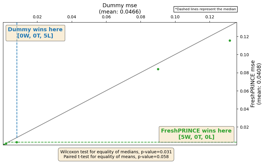
We can plot the results against each other. This also presents the wins and losses and some summary statistics.
[31]:
from aeon.visualisation import plot_pairwise_scatter

fig, ax = plot_pairwise_scatter(
    all_results[:, 1],
    all_results[:, 2],
    "FreshPRINCE",
    "Dummy",
    metric="mse",
    lower_better=True,
)
C:\Code\aeon\aeon\visualisation\results_plotting.py:476: UserWarning: This figure includes Axes that are not compatible with tight_layout, so results might be incorrect.
  fig.tight_layout()

Comparing multiple regressors
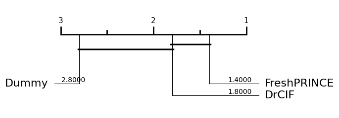
We can plot the results of multiple regressors on a critical difference diagram, which shows the average rank and groups estimators by whether they are significantly different from each other.
[33]:
from aeon.visualisation import plot_critical_difference

res = plot_critical_difference(
    all_results,
    regressors,
    lower_better=True,
)

[36]:
from aeon.visualisation import plot_boxplot_median

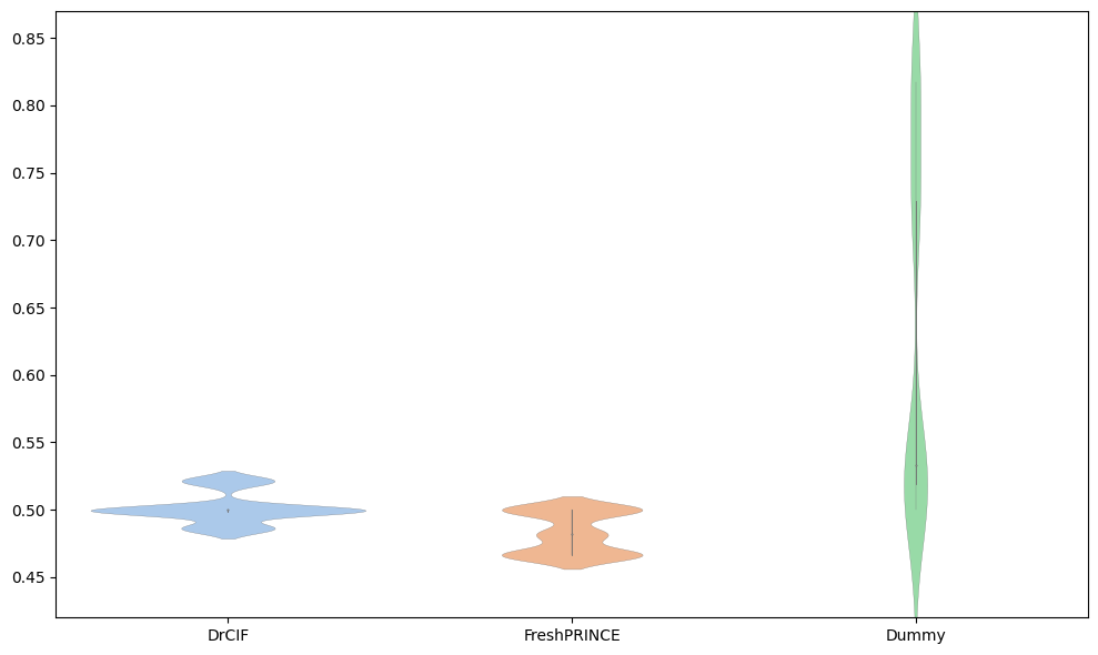
res = plot_boxplot_median(
    all_results,
    regressors,
)

Generated using nbsphinx. The Jupyter notebook can be found here.