Downloading and loading benchmarking datasets
It is common to use standard collections of data to compare different estimators for classification, clustering, regression, forecasting, and anomaly detection. Some of these datasets are shipped with aeon in the datasets/data directory. However, the files are far too big to include them all. aeon provides tools to download these data to use in benchmarking experiments. Classification and regression data are stored in .ts format. Forecasting data are stored in the equivalent .tsf format. Anomaly detection datasets are stored in the TimeEval .csv format. See the data loading notebook for more info.
Classification and regression are loaded into 3D numpy arrays of shape (n_cases, n_channels, n_timepoints) if equal length or a list of [n_cases] of 2D numpy if n_timepoints is different for different cases. Forecasting data are loaded into pd.DataFrame. Anomaly detection dataset are loaded into 2D numpy arrays of shape (n_timepoints, n_channels). For more information on aeon data types see the data structures notebook.
Note that this notebook is dependent on external websites, so will not function if you are not online or the associated website is down. We use the following four functions
[ ]:
from aeon.datasets import (
    load_anomaly_detection,
    load_classification,
    load_forecasting,
    load_regression,
)
Time Series Classification Archive
UCR/TSML Time Series Classification Archive hosts the UCR univariate TSC archive [1], also available from UCR and the multivariate archive [2] (previously called the UEA archive, soon to change). We provide seven of these in the datasets/data directory: ACSF1, ArrowHead, BasicMotions, GunPoint, ItalyPowerDemand, JapaneseVowels and PickupGestureWiimoteZ. The archive is much bigger. The last batch release was for 128 univariate [1] and 33 multivariate [2]. If you just want to download them all, please go to the website
[2]:
from aeon.datasets.tsc_datasets import multivariate, univariate

# This file also contains sub lists by type, e.g. unequal length
print("Univariate length = ", len(univariate))
print("Multivariate length = ", len(multivariate))
Univariate length =  128
Multivariate length =  30
A default train and test split is provided for this data. The file structure for a problem such as Chinatown is
<extract_path>/Chinatown/Chinatown_TRAIN.ts
<extract_path>/Chinatown/Chinatown_TEST.ts
You can load these problems directly from TSC.com and load them into memory. These functions can return associated metadata in addition to the data. This usage combines the train and test splits and loads them into one X and one y array.
[3]:
X, y, meta = load_classification("Chinatown", return_metadata=True)
print("Shape of X = ", X.shape)
print("First case = ", X[0][0], " has label = ", y[0])
print("\nMeta data = ", meta)
Shape of X =  (363, 1, 24)
First case =  [ 573.  375.  301.  212.   55.   34.   25.   33.  113.  143.  303.  615.
 1226. 1281. 1221. 1081.  866. 1096. 1039.  975.  746.  581.  409.  182.]  has label =  1

Meta data =  {'problemname': 'chinatown', 'timestamps': False, 'missing': False, 'univariate': True, 'equallength': True, 'classlabel': True, 'targetlabel': False, 'class_values': ['1', '2']}
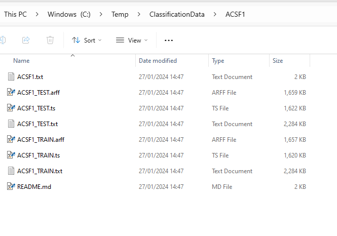
If you look in aeon/datasets you should see a directory called local_data containing the Chinatown datasets. All of the zips have .ts files. Some also have .arff and .txt files. File structure looks something like this:
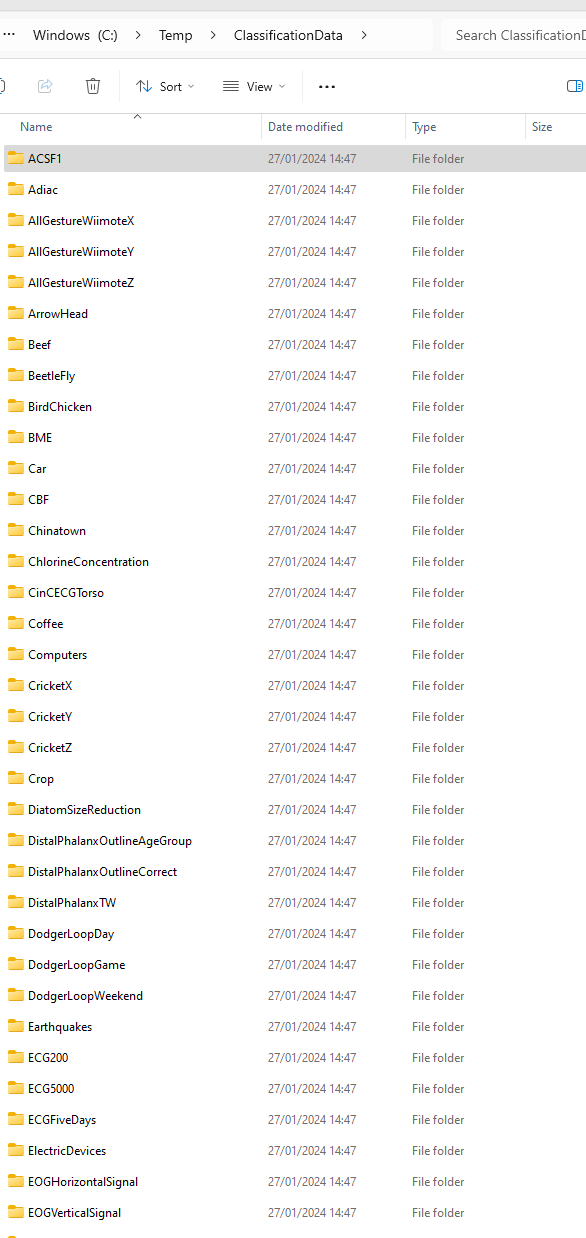
Within each folder are the data in text files formatted as .ts files (see the data loading notebook for file format description). They may also be available in .arff format and .txt format.
If you load again with the same extract path it will not download again if the file is already there. If you want to store data somewhere else, you can specify a file path. Also, you can load the train and test separately. This code will download the data to Temp once, and load into separate train/test splits. The split argument is not case sensitive. Once downloaded, load_classification is a equivalent to a call to load_from_ts_file
Time Series (Extrinsic) Regression
`The Monash Time Series Extrinsic Regression Archive <>`__ [3] repo (called extrinsic to differentiate if from sliding window based regression) currently contains 19 regression problems in .ts format. One of these, Covid3Month, is in datasets\data. We have recently expanded this repo to include 63 problems in .ts format. The usage of load_regression is identical to load_classification
[ ]:
from aeon.datasets.dataset_collections import get_available_tser_datasets

get_available_tser_datasets()
[5]:
X, y, meta = load_regression("FloodModeling1", return_metadata=True)
print("Shape of X = ", X.shape, " meta data = ", meta)
Shape of X = (673, 1, 266) meta data = {'problemname': 'floodmodeling1', 'timestamps': False, 'missing': False, 'univariate': True, 'equallength': True, 'classlabel': False, 'targetlabel': True, 'class_values': []}
Time Series Forecasting
The Monash time series forecasting repo contains a large number of forecasting data, including competition data such as M1, M3 and M4. Usage is the same as the other problems, although there is no provided train/test splits.
[6]:
from aeon.datasets.dataset_collections import get_available_tsf_datasets

get_available_tsf_datasets()
[6]:
['australian_electricity_demand_dataset',
 'car_parts_dataset_with_missing_values',
 'car_parts_dataset_without_missing_values',
 'cif_2016_dataset',
 'covid_deaths_dataset',
 'covid_mobility_dataset_with_missing_values',
 'covid_mobility_dataset_without_missing_values',
 'dominick_dataset',
 'elecdemand_dataset',
 'electricity_hourly_dataset',
 'electricity_weekly_dataset',
 'fred_md_dataset',
 'hospital_dataset',
 'kaggle_web_traffic_dataset_with_missing_values',
 'kaggle_web_traffic_dataset_without_missing_values',
 'kaggle_web_traffic_weekly_dataset',
 'kdd_cup_2018_dataset_with_missing_values',
 'kdd_cup_2018_dataset_without_missing_values',
 'london_smart_meters_dataset_with_missing_values',
 'london_smart_meters_dataset_without_missing_values',
 'm1_monthly_dataset',
 'm1_quarterly_dataset',
 'm1_yearly_dataset',
 'm3_monthly_dataset',
 'm3_other_dataset',
 'm3_quarterly_dataset',
 'm3_yearly_dataset',
 'm4_daily_dataset',
 'm4_hourly_dataset',
 'm4_monthly_dataset',
 'm4_quarterly_dataset',
 'm4_weekly_dataset',
 'm4_yearly_dataset',
 'nn5_daily_dataset_with_missing_values',
 'nn5_daily_dataset_without_missing_values',
 'nn5_weekly_dataset',
 'pedestrian_counts_dataset',
 'saugeenday_dataset',
 'solar_10_minutes_dataset',
 'solar_4_seconds_dataset',
 'solar_weekly_dataset',
 'sunspot_dataset_with_missing_values',
 'sunspot_dataset_without_missing_values',
 'tourism_monthly_dataset',
 'tourism_quarterly_dataset',
 'tourism_yearly_dataset',
 'traffic_hourly_dataset',
 'traffic_weekly_dataset',
 'us_births_dataset',
 'weather_dataset',
 'wind_4_seconds_dataset',
 'wind_farms_minutely_dataset_with_missing_values',
 'wind_farms_minutely_dataset_without_missing_values']
[7]:
X, metadata = load_forecasting("m4_yearly_dataset", return_metadata=True)
print(X.shape)
print(metadata)
data = X.head()
print(data)
(23000, 3)
{'frequency': 'yearly', 'forecast_horizon': 6, 'contain_missing_values': False, 'contain_equal_length': False}
  series_name     start_timestamp  \
0          T1 1979-01-01 12:00:00
1          T2 1979-01-01 12:00:00
2          T3 1979-01-01 12:00:00
3          T4 1979-01-01 12:00:00
4          T5 1979-01-01 12:00:00

                                        series_value
0  [5172.1, 5133.5, 5186.9, 5084.6, 5182.0, 5414....
1  [2070.0, 2104.0, 2394.0, 1651.0, 1492.0, 1348....
2  [2760.0, 2980.0, 3200.0, 3450.0, 3670.0, 3850....
3  [3380.0, 3670.0, 3960.0, 4190.0, 4440.0, 4700....
4  [1980.0, 2030.0, 2220.0, 2530.0, 2610.0, 2720....
Time Series Anomaly Detection (TSAD)
The TimeEval archive [5] contains 30 dataset collections for time series anomaly detection. Each collection consisting of many datasets from the same source. The collections are from a variety of domains, including cyber security, industrial processes, and healthcare. The datasets can directly be loaded using the load_anomaly_detection function:
[8]:
from aeon.datasets.tsad_datasets import multivariate, univariate

# This file also contains sub lists by learning type, e.g. semi-supervised, ...
print("Univariate length = ", len(univariate()))
print("Multivariate length = ", len(multivariate()))
Univariate length =  11233
Multivariate length =  342
A default train and test split is provided for all supervised and semi-supervised data. The file structure for a problem is
<extract_path>/<dimensionality>/<collection>/<dataset>.test.csv
<extract_path>/<dimensionality>/<collection>/<dataset>.train.csv
You can load these problems directly from the TimeEval archive [5] into memory. The loading function can also return associated metadata in addition to the data:
[9]:
name = ("Genesis", "genesis-anomalies")
X, y, meta = load_anomaly_detection(name, return_metadata=True)
print("Shape of X = ", X.shape)
print("Shape of y = ", y.shape)
print("\nMeta data = ", meta)
Shape of X =  (16220, 18)
Shape of y =  (16220,)

Meta data =  {'problemname': 'Genesis genesis-anomalies', 'timestamps': 16220, 'dimensions': 18, 'learning_type': 'unsupervised', 'contamination': 0.00308261405672, 'num_anomalies': 3}
References
[1] Dau et. al, The UCR time series archive, IEEE/CAA Journal of Automatica Sinica, 2019 [2] Ruiz et. al, The great multivariate time series classification bake off: a review and experimental evaluation of recent algorithmic advances, Data Mining and Knowledge Discovery 35(2), 2021 [3] Tan et. al, Time Series Extrinsic Regression, Data Mining and Knowledge Discovery, 2021 [4] Godahewa et. al, Monash Time Series Forecasting Archive,Neural Information Processing Systems Track on Datasets and Benchmarks, 2021 [5] Sebastian Schmidl, Phillip Wenig, Thorsten Papenbrock: Anomaly Detection in Time Series: A Comprehensive Evaluation. PVLDB 9:(15), 2022, DOI:10.14778/3538598.3538602.
[9]:
Generated using nbsphinx. The Jupyter notebook can be found here.
![]()