Time Series Similarity Search with aeon

The objectives of the similarity search module in aeon is to provide estimators with a fit/predict interface to solve the following use cases :

• Nearest neighbors search on time series subesequences or whole series

• Motifs search on time series subsequences

Similarly to the transformer module, the similarity_search module split estimators between series estimators and collection estimators, such as :

• series estimators take as input a single time series of shape (n_channels, n_timepoints) during fit and predict.

• collection estimators take as input a time series collection of shape (n_cases, n_channels, n_timepoints) during fit, and a single series of shape (n_channels, n_timepoints) during predict.

Note that the above is a general guideline, and that some estimators can also take None as input during predict, or series of length different to n_timepoints. We’ll explore the different estimators in the next sections.

Other similarity search notebooks

This notebook gives an overview of similarity search module and the available estimators. The following notebooks are also available to go more in depth with specific subject of similarity search in aeon:

• The theory and math behind the similarity search estimators in aeon

• Analysis of the performance of the estimators provided by similarity search module

# Define some plotting functions we'll use later !
def plot_best_matches(
    X_fit, X_predict, idx_predict, idx_matches, length, normalize=False
):
    """Plot the top best matches of a query in a dataset."""
    fig, ax = plt.subplots(figsize=(20, 5), ncols=len(idx_matches))
    if len(idx_matches) == 1:
        ax = [ax]
    for i_k, id_timestamp in enumerate(idx_matches):
        # plot the sample of the best match
        ax[i_k].plot(X_fit[0], linewidth=2)
        # plot the location of the best match on it
        match = X_fit[0, id_timestamp : id_timestamp + length]
        ax[i_k].plot(
            range(id_timestamp, id_timestamp + length),
            match,
            linewidth=7,
            alpha=0.5,
            color="green",
            label="best match location",
        )
        # plot the query on the location of the best match
        Q = X_predict[0, idx_predict : idx_predict + length]
        if normalize:
            Q = Q * np.std(match) + np.mean(match)
        ax[i_k].plot(
            range(id_timestamp, id_timestamp + length),
            Q,
            linewidth=5,
            alpha=0.5,
            color="red",
            label="query",
        )
        ax[i_k].set_title(f"best match {i_k}")
        ax[i_k].legend()
    plt.show()


def plot_matrix_profile(X, mp, i_k):
    """Plot the matrix profile and corresponding time series."""
    fig, ax = plt.subplots(figsize=(20, 10), nrows=2)
    ax[0].set_title("series X used to build the matrix profile")
    ax[0].plot(X[0])  # plot first channel only
    # This is necessary as mp is a list of arrays due to unequal length support
    # as it can have different number of matches for each step when
    # using threshold-based search.
    ax[1].plot([mp[i][i_k] for i in range(len(mp))])
    ax[1].set_title(f"Top {i_k+1} matrix profile of X")
    ax[1].set_ylabel(f"Dist to top {i_k+1} match")
    ax[1].set_xlabel("Starting index of the query in X")
    plt.show()

A word on base classes

All estimators of the similarity search module in aeon inherit from the BaseSimilaritySearch class, which define the some abstract methods that estimator must implement, such as fit and predict and some private function used to validate the format of the time series you will provide. Then, the two submodules series and collection also define a base class (BaseSeriesSimilaritySearch and BaseCollectionSeriesSearch) that their respective estimator will inherit from. If you ever want to extend the module or create your own estimators, these are the classes you’ll want to use to define the base structure of your estimator.

Load a dataset

In the following, we’ll use an easy dataset (ArrowHead) to help build intuition. Don’t hesitate to swap it with other datasets to explore ! We load it using the load_classification function.

import numpy as np
from matplotlib import pyplot as plt

from aeon.datasets import load_classification

# Load GunPoint dataset
X, y = load_classification("ArrowHead")

classes = np.unique(y)

fig, ax = plt.subplots(figsize=(20, 5), ncols=len(classes))
for i_class, _class in enumerate(classes):
    for i_x in np.where(y == _class)[0][0:2]:
        ax[i_class].plot(X[i_x, 0], label=f"sample {i_x}")
    ax[i_class].legend()
    ax[i_class].set_title(f"class {_class}")
plt.suptitle("Example samples for the GunPoint dataset")
plt.show()

1. Series estimators

First, we’ll explore estimators of the series module, where you must provide single series of shape (n_channels, n_timepoints) during fit.

1.1 Subsequence nearest neighbors with MASS

To perform nearest neighbors search on subsequences on a series, we can use the MassSNN estimator.

It takes as parameter during initialisation :

• length : an integer giving the length of the subsequences to extract from the series. It is also the expected length of the series given in predict

• normalize: a boolean indicating whether the subsequences should be independently z-normalized ((X-mean(X))/std(X)) before the distance computations. This results in a scale-independent matching.

To parameterize the search, additional parameters are available when calling the predict method:

• k (int) : the number of nearest neighbors to return.

• dist_threshold (float) : the maximum allowed distance for a candidate subsequence to be considered as a neighbor.

• allow_trivial_matches (bool) : whether a neighbors of a match to a query can be also considered as matches (True), or if an exclusion zone is applied around each match to avoid trivial matches with their direct neighbors (False).

• inverse_distance (bool) : if True, the matching will be made on the inverse of the distance, and thus, the farther neighbors will be returned instead of the closest ones.

• exclusion_factor (float): A factor of the length used to define the exclusion zone when allow_trivial_matches is set to False. For a given timestamp, the exclusion zone starts from id_timestamp - floor(length*exclusion_factor) and end at id_timestamp + floor(length*exclusion_factor).

• X_index (int): If series given during predict is a subsequence of series given during fit, specify its starting timestamp. If specified, neighboring subsequences of X won’t be able to match as neighbors.

First, we’ll select a series from the dataset to use during fit. This is the series we want our neighbors to come from.

from aeon.similarity_search.series import MassSNN

series_fit = X[2]
series_predict = X[3]

length = 50
snn = MassSNN(length=length, normalize=False).fit(series_fit)

plt.plot(series_fit[0], label="series fit")
plt.plot(series_predict[0], label="series predict")
plt.legend()
plt.show()
print(series_fit.shape)

(1, 251)

Then we’ll take a subsequence of size length in another series of the same class to use in predict :

starting_timestep_predict = 30

indexes, distances = snn.predict(
    series_predict[:, starting_timestep_predict : starting_timestep_predict + length],
    k=3,
    allow_trivial_matches=True,
)
for i in range(len(indexes)):
    print(f"match {i} : {indexes[i]} with distance {distances[i]}")
plot_best_matches(
    series_fit, series_predict, starting_timestep_predict, indexes, length
)

match 0 : 177 with distance 2.550008590853018
match 1 : 176 with distance 2.6262080735121316
match 2 : 31 with distance 2.7331649479116393

The predict method returns two lists, containing the starting timesteps of the matches in series_fit and the squared euclidean distance of these matches to the subsequence we gave in predict. Now, you can then play with the different parameters of predict to customize your search results to your needs!

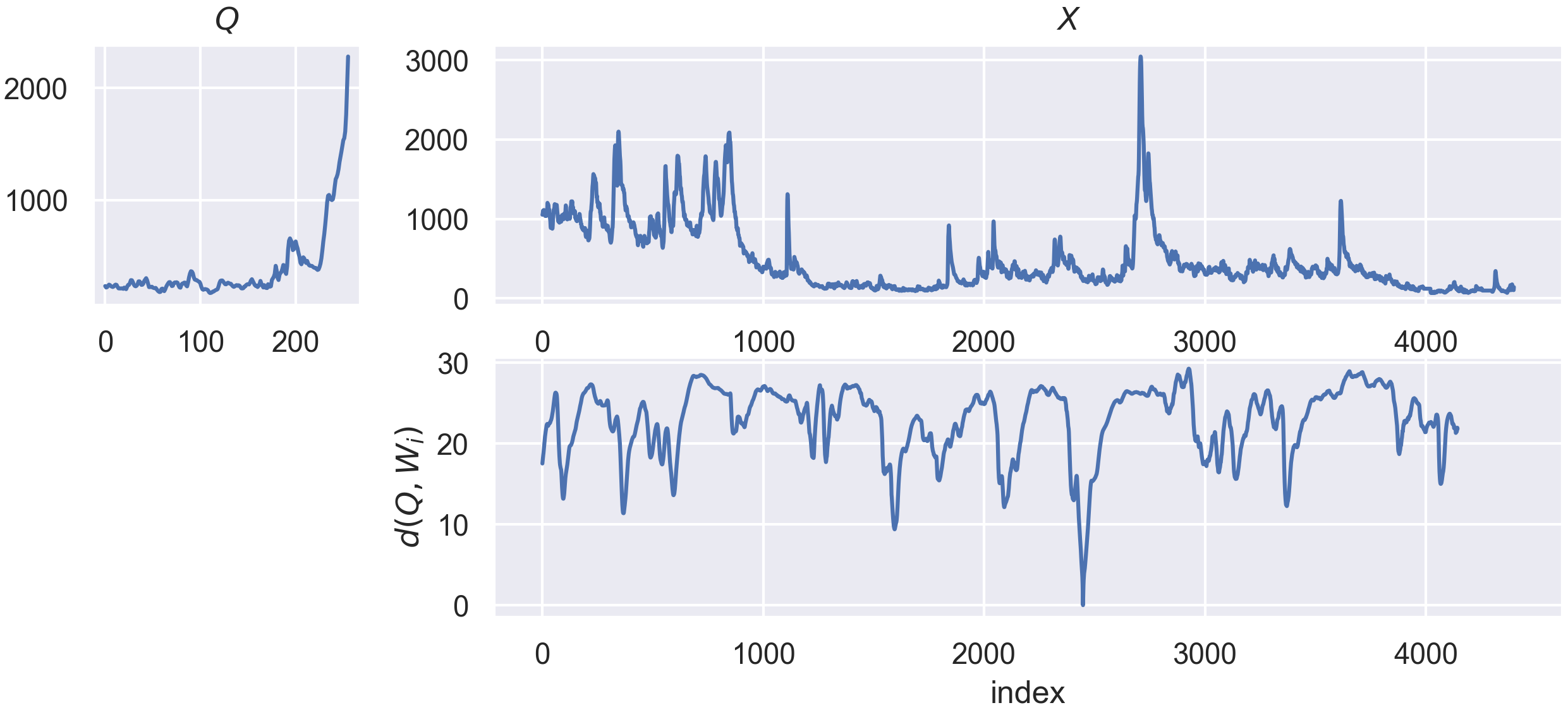
It is also possible to get the distance profile which is used to extract the best matches :

distance_profile = snn.compute_distance_profile(
    series_predict[:, starting_timestep_predict : starting_timestep_predict + length],
)
plt.figure(figsize=(7, 2))
plt.plot(distance_profile)
plt.show()

1.2 Motif search with StompMotif estimator

When doing motif search, it’s important to define the type of motif you want to extract from a series. We’ll use the figure and definitions given by [1] and make some adjustment to clear out some confusion due to the naming of each method:

For now, the StompMotif estimators supports only the following configuration, which you will have to specify using the parameters of the predict method :

• for “Pair Motifs” : This is the default configuration with {"motif_size": 1}, meaning we extract the closest match to each candidate, so we end up with the pair (candidate, closest match)

• for “k-motif”, which we define as the extension of Pair motifs to : {"motif_size": k}. For k=2, we would extract (candidate, closest match 1, closest match 2)

• for “r-motifs”, which we renamed from k-motif in the figure, because it is a range-based method : {"motif_size": np.inf, "dist_threshold":  r, "motif_extraction_method": "r_motifs"}

These configuration will extract the best motif only, if you want to extract more than one motifs, you can use the k parameter to extract the top-k motifs.

The term ``k`` of ``top-k`` motifs, while also used in ``k-motifs``, is not the same. To avoid confusion of both terms, we use ``motif_size`` instead of ``k`` to specify the size of the motifs to extract. This avoids the phrasing “extracting the ``top-k`` ``k-motif``”, which would be confusing and ill defined. Rather, we extract the ``top-k`` ``motif_size-motifs``.

The top-k using motif_extraction_method="r_motifs" will be the motifs with the highest cardinality (i.e. the more matches in range r), while for motif_extraction_method="k_motifs",which is the default value, the best motifs will be those who minimize the maximum pairwise distance.

from aeon.similarity_search.series import StompMotif

motif = StompMotif(length=length, normalize=True)
motif.fit_predict(series_fit, k=3, motif_size=1)

([array([[ 40, 192]]), array([[192,  40]]), array([[158,   8]])],
 [array([0.21749257]), array([0.21749257]), array([0.23961497])])

The above use of fit_predict is equivalent to the following calls, with is_self_computation=True indicating that the series in fit is the same that the series in predict, so it shouldn’t match the same subsequences as motifs :

motif = StompMotif(length=length, normalize=True)
motif.fit(series_fit)
motif.predict(series_fit, k=3, motif_size=1, is_self_computation=True)

([array([[ 40, 192]]), array([[192,  40]]), array([[158,   8]])],
 [array([0.21749257]), array([0.21749257]), array([0.23961497])])

While the above example only use series_fit to search motifs in the same series, we also support giving another series in predict, which will use this series to search for the motifs matching subsequences in the series given during fit. For those familiar with the matrix profile notations, this is the case of using MP(A,B), while not using a series in predict is doing a self matrix profile MP(A,A).

from aeon.similarity_search.series import StompMotif

motif.predict(
    series_predict,
    k=3,
    motif_size=1,
)

([array([[149,   4]]), array([[ 62, 201]]), array([[3, 5]])],
 [array([0.15686187]), array([0.27831027]), array([0.29831867])])

You can also return the matrix profile with the same parameterization as predict (minus motif_extraction_method parameter) using :

MP, IP = motif.compute_matrix_profile(series_predict)

plt.figure(figsize=(7, 2))
plt.plot([MP[i][0] for i in range(len(MP))])
plt.show()

2. Collection estimators

Now, we’ll explore estimators of the collection module, where you must provide single series of shape (n_cases, n_channels, n_timepoints) during fit and predict.

This method uses a random projection locality sensitive hashing index based on cosine similarity. We define a hash function as a boolean operation such as, given a random vector V of shape (n_channels, L) and a time series X of shape (n_channels, n_timeponts) (with L<=n_timepoints), we compute X.V > 0 to obtain hash of X

In the case where L<n_timepoints, each hash function is affected a starting point s (between [0, n_timepoints - L]) to compute X[:, s:s+L].V > 0 instead.

The RandomProjectionIndexANN estimators use the parameter n_hash_funcs to create that much random hash function as defined above. Each series X of the collection given in fit is then represented as an array of n_hash_funcs boolean, which is then hashed to a dictionary as {hash(bool_arry): case_id_array}.

To compute the nearest neighbors of a series X given in predict, we first transform this series to a boolean array using our previously defined hash functions, and then use the result of hash(bool_array) to look at the bucket in which X falls, and consider the case_id_array as the indexes of its neighbors. If this bucket doesn’t exists, we compute a distance matrix between the boolean array of X and every boolean array making the keys of the dictionary to get similar buckets.

This method will not provide exact results, but will perform approximate searches. This also ignore any temporal correlation and consider series as high dimensional points due to the cosine similarity distance.

from aeon.similarity_search.collection import RandomProjectionIndexANN

X_fit = X[:-2]
# we use a single series for this example but it will be converted into a collection
# as this is a collection estimators.
X_predict = X[-1]
index = RandomProjectionIndexANN().fit(X_fit)
indexes, distances = index.predict(X_predict, k=3)
# as X_predict is converted to a collection, we select the first returns
# to obtain its results
indexes = indexes[0]
distances = distances[0]

for i in range(len(indexes)):
    print(f"match {i} : {indexes[i]} with distance {distances[i]}")
    # A bit of hacking of the function defined for series estimator to show best matches
    plot_best_matches(X_fit[indexes[i]], X_predict, 0, [0], X_predict.shape[1])

match 0 : 32 with distance 1.0

match 1 : 159 with distance 2.0

match 2 : 203 with distance 2.0

You can then play with the different parameter of the estimator to affect the speed vs accuracy of the index, for example increasing n_hash_funcs from the default 128 to 512, and considering larger vectors (V of shape (n_channels, L)) for the hash functions by tuning hash_func_coverage (a float between 0 and 1, with 0.25 as default) such as L = n_timepoints * hash_func_coverage:

index = RandomProjectionIndexANN(n_hash_funcs=512, hash_func_coverage=0.75).fit(X_fit)
indexes, distances = index.predict(X_predict, k=2)

indexes = indexes[0]
distances = distances[0]

for i in range(len(indexes)):
    print(f"match {i} : {indexes[i]} with distance {distances[i]}")
    # A bit of hacking of the function defined for series estimator to show best matches
    plot_best_matches(X_fit[indexes[i]], X_predict, 0, [0], X_predict.shape[1])

match 0 : 17 with distance 12.0

match 1 : 190 with distance 13.0

This type of method is mostly interesting where speed of the search is paramount, or when the dataset size grows large (> 10k samples).

[1] Patrick Schäfer and Ulf Leser. 2022. Motiflets: Simple and Accurate Detection of Motifs in Time Series. Proc. VLDB Endow. 16, 4 (December 2022), 725–737.

---

Generated using nbsphinx. The Jupyter notebook can be found here.