Analysis of the speedups provided by similarity search module

In this notebook, we will explore the gains in time and memory of the different methods we use in the similarity search module.

import numpy as np
import pandas as pd
import seaborn as sns
from matplotlib import pyplot as plt

from aeon.similarity_search.distance_profiles._commons import (
    rolling_window_stride_trick,
)
from aeon.utils.numba.general import sliding_mean_std_one_series

sns.set()
sns.set_context()

Computing means and standard deviations for all subsequences

When we want to compute a normalized distance, given a time series X of size m and a query q of size l, we have to compute the mean and standard deviation for all subsequences of size l in X. One could do this task by doing the following:

def get_means_stds(X, q_length):
    windows = rolling_window_stride_trick(X, q_length)
    return windows.mean(axis=-1), windows.std(axis=-1)


rng = np.random.default_rng()
size = 100
q_length = 10

# Create a random series with 1 feature and 'size' timesteps
X = rng.random((1, size))
means, stds = get_means_stds(X, q_length)
print(means.shape)

(1, 91)

One issue with this code is that it actually recompute a lot of information between the computation of mean and std of each windows. Suppose that the window we compute the mean for W_i = {x_i, ..., x_{i+(l-1)}, to do this, we sum all the elements and divide them by l. You then want to compute the mean for W_{i+1} = {x_{i+1}, ..., x_{i+1+(l-1)}, which shares most of its values with W_i expect for x_i and x_{i+1+(l-1).

The optimization here consists in keeping a rolling sum, we only compute the full sum of the l values for the first window W_0, then to obtain the sum for W_1, we remove x_0 and add x_{1+(l-1)} from the sum of W_0. We can also a rolling squared sum to compute the standard deviation.

The sliding_mean_std_one_series function implement the computation of the means and standard deviations using these two rolling sums. The last argument indicates the dilation to apply to the subsequence, which is not used here, hence the value of 1 in the code bellow.

sizes = [500, 1000, 5000, 10000, 50000]
q_lengths = [50, 100, 250, 500]
times = pd.DataFrame(
    index=pd.MultiIndex(levels=[[], []], codes=[[], []], names=["size", "q_length"])
)
# A first run for numba compilations if needed
sliding_mean_std_one_series(rng.random((1, 50)), 10, 1)
for size in sizes:
    for q_length in q_lengths:
        X = rng.random((1, size))
        _times = %timeit -r 7 -n 10 -q -o get_means_stds(X, q_length)
        times.loc[(size, q_length), "full computation"] = _times.average
        _times = %timeit -r 7 -n 10 -q -o sliding_mean_std_one_series(X, q_length, 1)
        times.loc[(size, q_length), "sliding_computation"] = _times.average

fig, ax = plt.subplots(ncols=len(q_lengths), figsize=(20, 5), dpi=200)
for j, (i, grp) in enumerate(times.groupby("q_length")):
    grp.droplevel(1).plot(label=i, ax=ax[j])
    ax[j].set_title(f"query length {i}")
ax[0].set_ylabel("time in seconds")
plt.show()

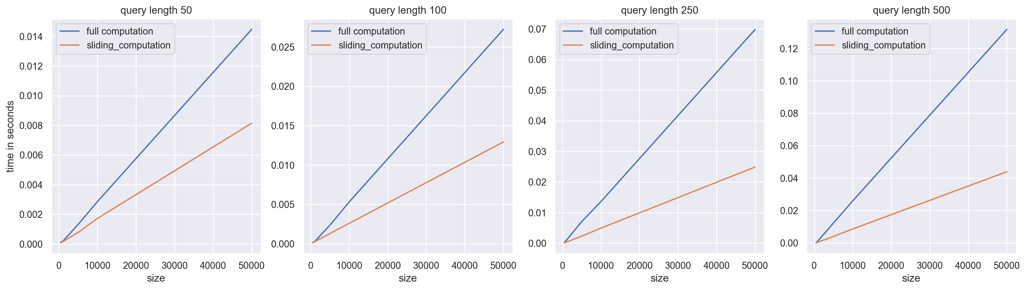
As you can see, the larger the size of q, the greater the speedups. This is because the larger the size of q, the more recomputation we avoid by using a sliding sum.

---

Generated using nbsphinx. The Jupyter notebook can be found here.