Benchmarking: retrieving and comparing against published results

You can access all archived published results for time series classification (TSC) directly with aeon. These results are all stored on the website timeseriesclassification.com. Coming soon, equivalent results for clustering and classification. These are reference results and will not change. The mechanism for recovering these results is intentionally hard coded and not generalised, to remove any potential for confusion. To more flexibly load the latest results for classification, clustering and regression, see the notebook Loading reference results.

These results were presented in three bake offs for classification: The first bake off [1] used 85 UCR univariate TSC datasets. The second bake off [2] introduced the multivariate TSC archive, and compared classifier performance. The third bake off [3], the bake off redux, compared univariate classifiers on 112 UCR datasets. Note the third bake off, or bake off redux as we call it, introduced 30 new datasets. These data and results for them will be available if the paper is accepted for publication.

We provide dictionary of classifier/index in results used in each bake off in the file aeon.benchmarking.results_loaders.

We compare results with the critical difference graph described in the benchmarking documentation. Note that the way we group classifiers has slightly changed and hence there may be small variation in cliques from published results.

The published results for two bake offs can be recovered from time series repo directly or with aeon.

The great time series classification bake off, 2017

The first TSC bake off, conducted in 2015 and published in 2017 compared 25 classifiers on the 85 UCR data that were released in 2015. The classifiers used are:

from aeon.benchmarking.results_loaders import uni_classifiers_2017

print(uni_classifiers_2017.keys())

dict_keys(['ACF', 'BOSS', 'CID_DTW', 'CID_ED', 'DDTW_R1_1NN', 'DDTW_Rn_1NN', 'DTW_F', 'EE', 'ERP_1NN', 'Euclidean_1NN', 'FlatCOTE', 'FS', 'LCSS_1NN', 'LPS', 'LS', 'MSM_1NN', 'PS', 'RotF', 'SAXVSM', 'ST', 'TSBF', 'TSF', 'TWE_1NN', 'WDDTW_1NN', 'WDTW_1NN'])

The dataset used for the first bake off [1] are described in [4] and listed as uni_classifiers_2017. They are listed as:

from aeon.datasets.tsc_datasets import univariate2015

print(
    f"The {len(univariate2015)} UCR univariate datasets described in [4] and used in "
    f"2017 bakeoff [1]:\n{univariate2015}"
)

The 85 UCR univariate datasets described in [4] and used in 2017 bakeoff [1]:
{'MiddlePhalanxTW', 'TwoLeadECG', 'WormsTwoClass', 'Meat', 'MiddlePhalanxOutlineCorrect', 'Beef', 'ArrowHead', 'ECG5000', 'ScreenType', 'Wine', 'Adiac', 'Coffee', 'DistalPhalanxOutlineCorrect', 'OliveOil', 'Symbols', 'Lightning2', 'SonyAIBORobotSurface2', 'Computers', 'Haptics', 'UWaveGestureLibraryY', 'FacesUCR', 'SwedishLeaf', 'WordSynonyms', 'ProximalPhalanxTW', 'ProximalPhalanxOutlineAgeGroup', 'ShapeletSim', 'Herring', 'Car', 'CricketY', 'UWaveGestureLibraryZ', 'Phoneme', 'PhalangesOutlinesCorrect', 'HandOutlines', 'InlineSkate', 'SyntheticControl', 'Yoga', 'ProximalPhalanxOutlineCorrect', 'ToeSegmentation2', 'Ham', 'CricketZ', 'Trace', 'Worms', 'UWaveGestureLibraryAll', 'CricketX', 'DiatomSizeReduction', 'FordA', 'CinCECGTorso', 'MedicalImages', 'FaceAll', 'Plane', 'ToeSegmentation1', 'RefrigerationDevices', 'OSULeaf', 'MoteStrain', 'ShapesAll', 'CBF', 'ECG200', 'Lightning7', 'SonyAIBORobotSurface1', 'SmallKitchenAppliances', 'FordB', 'ECGFiveDays', 'TwoPatterns', 'DistalPhalanxOutlineAgeGroup', 'LargeKitchenAppliances', 'NonInvasiveFetalECGThorax2', 'Mallat', 'DistalPhalanxTW', 'ItalyPowerDemand', 'GunPoint', 'NonInvasiveFetalECGThorax1', 'Earthquakes', 'ChlorineConcentration', 'Wafer', 'Fish', 'ElectricDevices', 'StarlightCurves', 'InsectWingbeatSound', 'FiftyWords', 'BirdChicken', 'MiddlePhalanxOutlineAgeGroup', 'Strawberry', 'BeetleFly', 'UWaveGestureLibraryX', 'FaceFour'}

You can pull down results for the original bake off for either the default train/test split and for results averaged over 100 resamples.

from aeon.benchmarking.results_loaders import get_bake_off_2017_results

default = get_bake_off_2017_results()
averaged = get_bake_off_2017_results(default_only=False)
print(
    f"{len(univariate2015)} datasets in rows, {len(uni_classifiers_2017)} classifiers "
    f"in columns"
)

85 datasets in rows, 25 classifiers in columns

Once you have the results you want, you can compare classifiers with built in aeon tools.

Suppose we want to recreate the critical difference diagram published in [1]:

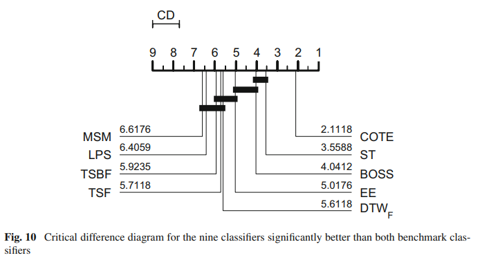
This displays the critical difference diagram [6] for comparing classifiers. It shows the average rank of each estimator over all datasets. It then groups estimators for which there is no significant difference in rank into cliques, shown with a solid bar. The published results used the original method for finding cliques called the post hoc Nemenyi test. Our plotting tool offers this as an alternative. See the docs for aeon.visualisation.plot_critical_difference for more details. To recreate the above, we can do this (note slight difference in names, MSM_1NN is MSM and FlatCOTE is COTE.

from aeon.visualisation import plot_critical_difference

classifiers = ["MSM_1NN", "LPS", "TSBF", "TSF", "DTW_F", "EE", "BOSS", "ST", "FlatCOTE"]
# Get columm positions of classifiers in results
indx = [uni_classifiers_2017[key] for key in classifiers if key in uni_classifiers_2017]
plot, _ = plot_critical_difference(averaged[:, indx], classifiers, test="Nemenyi")
plot.show()

C:\Users\Tony\AppData\Local\Temp\ipykernel_26644\1537479541.py:7: UserWarning: Matplotlib is currently using module://matplotlib_inline.backend_inline, which is a non-GUI backend, so cannot show the figure.
  plot.show()

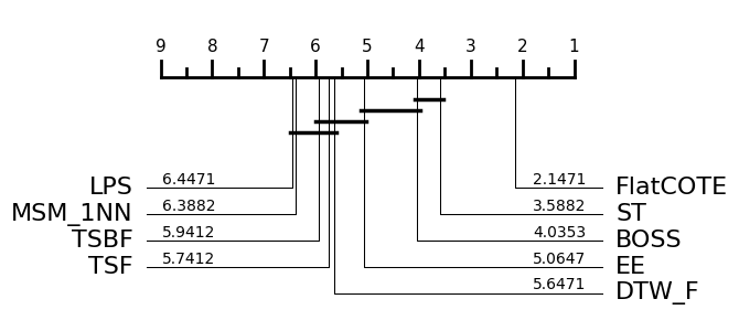
Note there are some small differences in averaged rank. This may be due to differences in how ties in rank were handled. The cliques are identical. Given that these results were generated in 2014/2015 and matlab was used to draw the diagrams, we think this is an acceptable reproduction. Subsequent to the 2015 bake off we switched to using pairwise Wilcoxon sign rank tests with the Holm correction. This creates slightly different cliques.

The great multivariate time series classification bake off [2], 2021

Link to paper

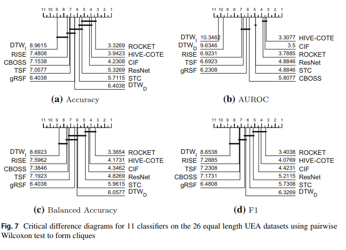
The multivariate bake off [2] launched a new archive and compared 11 classifiers on 26 multivariate TSC problems

from aeon.benchmarking.results_loaders import multi_classifiers_2021
from aeon.datasets.tsc_datasets import multivariate_equal_length

print(multi_classifiers_2021.keys())
print(
    f"The {len(multivariate_equal_length)} TSML multivariate datasets described in "
    f"and used in the 2021 multivariate bakeoff [1]:\n{multivariate_equal_length}"
)

dict_keys(['CBOSS', 'CIF', 'DTW_D', 'DTW_I', 'gRSF', 'HIVE-COTEv1', 'ResNet', 'RISE', 'ROCKET', 'STC', 'TSF'])
The 26 TSML multivariate datasets described in and used in the 2021 multivariate bakeoff [1]:
{'FaceDetection', 'Handwriting', 'Cricket', 'UWaveGestureLibrary', 'AtrialFibrillation', 'SelfRegulationSCP2', 'DuckDuckGeese', 'SelfRegulationSCP1', 'Epilepsy', 'Libras', 'BasicMotions', 'MotorImagery', 'PenDigits', 'PhonemeSpectra', 'StandWalkJump', 'PEMS-SF', 'Heartbeat', 'EthanolConcentration', 'ArticularyWordRecognition', 'LSST', 'FingerMovements', 'NATOPS', 'EigenWorms', 'ERing', 'RacketSports', 'HandMovementDirection'}

The results table below shows the performance figures for accuracy, balanced accuracy, AUROC and F1.

We can recreate the accuracy graph by loading the results from tsc.com and plotting like so:

from aeon.benchmarking.results_loaders import get_bake_off_2021_results

default = get_bake_off_2021_results()
averaged = get_bake_off_2021_results(default_only=False)
print("Shape of results = ", averaged.shape)

Shape of results =  (26, 11)

plot, _ = plot_critical_difference(averaged, list(multi_classifiers_2021.keys()))

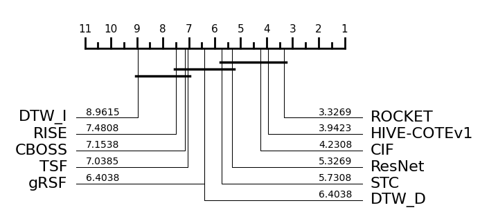
Note there are some differences in cliques due to slightly different methodology. This will be explained in more detail in a technical document soon. We will also add more reference results in due course.

---

Generated using nbsphinx. The Jupyter notebook can be found here.