plot_critical_difference
- plot_critical_difference(scores: ndarray | list, labels: list[str], highlight: dict[str, str] | None = None, lower_better: bool = False, test: str = 'wilcoxon', correction: str = 'holm', alpha: float = 0.1, width: float = 6, textspace: float = 1.5, reverse: bool = True, return_p_values: bool = False) tuple[Figure, Axes] | tuple[Figure, Axes, ndarray][source]
Plot the average ranks and cliques based on the method described in [1].
This function summarises the relative performance of multiple estimators evaluated on multiple datasets. The resulting plot shows the average rank of each estimator on a number line. Estimators are grouped by solid lines, called cliques. A clique represents a group of estimators within which there is no significant difference in performance (see the caveats below). Please note that these diagrams are not an end in themselves, but rather form one part of the description of performance of estimators.
The input is a summary performance measure of each estimator on each problem, where columns are estimators and rows datasets. This could be any measure such as accuracy/error, F1, negative log-likelihood, mean squared error or rand score.
This algorithm first calculates the rank of all estimators on all problems ( averaging ranks over ties), then sorts estimators on average rank. It then forms cliques. The original critical difference diagrams [1] use the post hoc Neymeni test [Rbf00f587966d-4] to find a critical difference. However, as discussed [Rbf00f587966d-3],this post hoc test is sensitive to the estimators included in the test: “For instance the difference between A and B could be declared significant if the pool comprises algorithms C, D, E and not significant if the pool comprises algorithms F, G, H.”. Our default option is to base cliques finding on pairwise Wilcoxon sign rank test.
There are two issues when performing multiple pairwise tests to find cliques: what adjustment to make for multiple testing, and whether to perform a one sided or two sided test. The Bonferroni adjustment is known to be conservative. Hence, by default, we base our clique finding from pairwise tests on the control tests described in [1] and the sequential method recommended in [Rbf00f587966d-2] and proposed in [Rbf00f587966d-5] that uses a less conservative adjustment than Bonferroni.
We perform all pairwise tests using a one-sided Wilcoxon sign rank test with the Holm correction to alpha, which involves reducing alpha by dividing it by number of estimators -1.
Suppose we have four estimators, A, B, C and D sorted by average rank. Starting from A, we test the null hypothesis that average ranks are equal against the alternative hypothesis that the average rank of A is less than that of B, with significance level alpha/(n_estimators-1). If we reject the null hypothesis then we stop, and A is not in a clique. If we cannot reject the null, we test A vs C, continuing until we reject the null or we have tested all estimators. Suppose we find that A vs B is significant. We form no clique for A.
We then continue to form a clique using the second best estimator, B, as a control. Imagine we find no difference between B and C, nor any difference between B and D. We have formed a clique for B: [B, C, D]. On the third iteration, imagine we also find not difference between C and D and thus form a second clique, [C, D]. We have found two cliques, but [C,D] is contained in [B, C, D] and is thus redundant. In this case we would return a single clique, [B, C, D].
Not this is a heuristic approach not without problems: If the best ranked estimator A is significantly better than B but not significantly different to C, this will not be reflected in the diagram. Because of this, we recommend also reporting p-values in a table, and exploring other ways to present results such as pairwise plots. Comparing estimators on archive data sets can only be indicative of overall performance in general, and such comparisons should be seen as exploratory analysis rather than designed experiments to test an a priori hypothesis.
Parts of the code are adapted from https://github.com/hfawaz/cd-diagram with permission from the owner.
- Parameters:
- scoresnp.array
Performance scores for estimators of shape (n_datasets, n_estimators).
- labelslist of estimators
List with names of the estimators. Order should be the same as scores
- highlightdict, default = None
A dict with labels and HTML colours to be used for highlighting. Order should be the same as scores.
- lower_betterbool, default = False
Indicates whether smaller is better for the results in scores. For example, if errors are passed instead of accuracies, set
lower_bettertoTrue.- teststring, default = “wilcoxon”
test method used to form cliques, either “nemenyi” or “wilcoxon”
- correction: string, default = “holm”
correction method for multiple testing, one of “bonferroni”, “holm” or “none”.
- alphafloat, default = 0.1
Critical value for statistical tests of difference.
- widthint, default = 6
Width in inches.
- textspaceint
Space on figure sides (in inches) for the method names (default: 1.5).
- reversebool, default = True
If set to ‘True’, the lowest rank is on the right.
- return_p_valuesbool, default = False
Whether to return the pairwise matrix of p-values.
- Returns:
- figmatplotlib.figure.Figure
- axmatplotlib.axes.Axes
- p_valuesnp.ndarray (optional)
if return_p_values is True, returns a (n_estimators, n_estimators) matrix of unadjusted p values for the pairwise Wilcoxon sign rank test.
References
Journal of Machine Learning Research 7:1-30, 2006. .. [Rbf00f587966d-2] García S. and Herrera F., “An extension on “statistical comparisons of classifiers over multiple data sets” for all pairwise comparisons.” Journal of Machine Learning Research 9:2677-2694, 2008. .. [Rbf00f587966d-3] Benavoli A., Corani G. and Mangili F “Should we really use post-hoc tests based on mean-ranks?” Journal of Machine Learning Research 17:1-10, 2016. .. [Rbf00f587966d-4] Nemenyi P., “Distribution-free multiple comparisons”. PhD thesis, Princeton University, 1963. .. [Rbf00f587966d-5] Holm S., “ A simple sequentially rejective multiple test procedure.” Scandinavian Journal of Statistics, 6:65-70, 1979.
Examples
>>> from aeon.visualisation import plot_critical_difference
>>> from aeon.benchmarking.results_loaders import get_estimator_results_as_array
>>> methods = ["IT", "WEASEL-Dilation", "HIVECOTE2", "FreshPRINCE"]
>>> results = get_estimator_results_as_array(estimators=methods)
>>> plot = plot_critical_difference(results[0], methods, alpha=0.1)
>>> plot.show()
>>> plot.savefig("cd.pdf", bbox_inches="tight")