Provided datasets

aeon ships several example data sets for machine learning tasks in the module datasets. This notebook gives an overview of what is available by default. For downloading data from other archives, see the loading data from web notebook. For further details on the form of the data, see the data loading notebook.

Forecasting

Forecasting data are stored in csv files with a header for column names. Six standard example datasets are shipped by default:

dataset name	loader function	properties
Box/Jenkins airline data	load_airline	univariate
Lynx sales data	load_lynx	univariate
Shampoo sales data	load_shampoo_sales	univariate
Pharmaceutical Benefit Scheme data	load_PBS_dataset	univariate
Longley US macroeconomic data	load_longley	multivariate
MTS consumption/income data	load_uschange	multivariate

These are stored in csv format in time, value format, including a header. For forcasting files, each column that is not an index is considered a time series. For example, the airline data has a single time series each row a time, value pair:

Date,Passengers
1949-01,112
1949-02,118

Longley has seven time series, each in its own column. Each row is the same time index:

"Obs","TOTEMP","GNPDEFL","GNP","UNEMP","ARMED","POP","YEAR"
1,60323,83,234289,2356,1590,107608,1947
2,61122,88.5,259426,2325,1456,108632,1948
3,60171,88.2,258054,3682,1616,109773,1949

The problem specific loading functions return the series as either a pd.Series if a single series or, if multiple series, a pd.DataFrame with each column a series. There are currently six forecasting problems shipped.

Airline

The classic Box & Jenkins airline data. Monthly totals of international airline passengers, 1949 to 1960. This data shows an increasing trend, non-constant (increasing) variance and periodic, seasonal patterns. The

import warnings

from aeon.datasets import load_airline
from aeon.visualisation import plot_series

warnings.filterwarnings("ignore")

airline = load_airline()
plot_series(airline)

(<Figure size 1600x400 with 1 Axes>,
 <Axes: ylabel='Number of airline passengers'>)

Longley

This mulitvariate time series dataset contains various US macroeconomic variables from 1947 to 1962 that are known to be highly collinear. This loader returns the series to be forecast (default TOTEMP: total employment) and other variables that may be useful in the forecast GNPDEFL - Gross national product deflator GNP - Gross national product UNEMP - Number of unemployed ARMED - Size of armed forces POP - Population

from aeon.datasets import load_longley

employment, longley = load_longley()
plot_series(employment)

(<Figure size 1600x400 with 1 Axes>, <Axes: ylabel='TOTEMP'>)

Lynx

The annual numbers of lynx trappings for 1821–1934 in Canada. This time-series records the number of skins of predators (lynx) that were collected over several years by the Hudson’s Bay Company. Returns a pd.Series

from aeon.datasets import load_lynx

lynx = load_lynx()
plot_series(lynx)

(<Figure size 1600x400 with 1 Axes>, <Axes: ylabel='Number of Lynx trappings'>)

PBS_dataset

The Pharmaceutical Benefits Scheme (PBS) is the Australian government drugs subsidy scheme. Data comprises of the numbers of scripts sold each month for immune sera and immunoglobulin products in Australia. The load function returns a pd.Series.

from aeon.datasets import load_PBS_dataset

pbs = load_PBS_dataset()
plot_series(pbs)

(<Figure size 1600x400 with 1 Axes>, <Axes: ylabel='Number of scripts'>)

ShampooSales

ShampooSales contains a single monthly time series of the number of sales of shampoo over a three year period. The units are a sales count.

from aeon.datasets import load_shampoo_sales

shampoo = load_shampoo_sales()
print(type(shampoo))
plot_series(shampoo)

<class 'pandas.core.series.Series'>

(<Figure size 1600x400 with 1 Axes>, <Axes: ylabel='Number of shampoo sales'>)

UsChange

Load MTS dataset for forecasting Growth rates of personal consumption and income. The data is quarterly for 188 quarters and contains time series for Consumption, Income, Production, Savings and Unemployment. It returns a pd.Series to forecast (by default, the series Consumption) and a pd.DataFrame containing the other series.

from aeon.datasets import load_uschange

consumption, others = load_uschange()
print(type(consumption))
plot_series(consumption)

<class 'pandas.core.series.Series'>

(<Figure size 1600x400 with 1 Axes>, <Axes: ylabel='Consumption'>)

Solar

Example national solar data for the GB eletricity network extracted from the Sheffield Solar PV_Live API. Note that these are estimates of the true solar generation, since the true values are “behind the meter” and essentially unknown. The returned pandas DataSeries is half hourly.

from aeon.datasets import load_solar

solar = load_solar()
print(type(solar))
plot_series(solar)

<class 'pandas.core.series.Series'>

(<Figure size 1600x400 with 1 Axes>, <Axes: ylabel='solar_gen'>)

Time series clustering, classification and regression

We ship several datasets from the UCR/TSML archives. The complete archives (including these examples) are available at the time series classification site and the UCR classification and clustering site. All the archive data can be loaded from these websites or directly from the web in code, see data downloads. All data is provided with a default train, test split. Problem loaders have an argument split. If not set, the function returns the combined train and test data. If split is set to "test" or "train", the required split is return. split is not case sensitive. They can also be loaded with the functions load_classification and load_regression, which also return meta data. See the notebook data loading for details. The data X is stored in a 3D numpy array of shape (n_cases, n_channels, n_timepoints) unless unequal length, in which case a list of 2D numpy array is returned.

dataset name	loader function	properties
Appliance power consumption	load_acsf1	univariate, equal length/index
Arrowhead shape	load_arrow_head	univariate, equal length/index
Gunpoint motion	load_gunpoint	univariate, equal length/index
Italy power demand	load_italy_power_demand	univariate, equal length/index
Japanese vowels	load_japanese_vowels	univariate, unequal length/index
OSUleaf leaf shape	load_osuleaf	univariate, equal length/index
Basic motions	load_basic_motions	multivariate, equal length/index

ACSF1

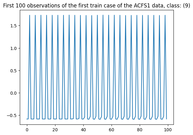
The dataset is compiled from ACS-F1, the first version of the database of appliance consumption signatures. The dataset contains the power consumption of typical appliances. The recordings are characterized by long idle periods and some high bursts of energy consumption when the appliance is active.

The classes correspond to 10 categories of home appliances: mobile phones (via chargers), coffee machines, computer stations (including monitor), fridges and freezers, Hi-Fi systems (CD players), lamp (CFL), laptops (via chargers), microwave ovens, printers, and televisions (LCD or LED).

The problem is univariate and equal length. It has high frequency osscilation.

import matplotlib.pyplot as plt

from aeon.datasets import load_acsf1

trainX, trainy = load_acsf1(split="train")
testX, testy = load_acsf1(split="test")
print(type(trainX))
print(trainX.shape)
plt.plot(trainX[0][0][:100])
plt.title(
    f"First 100 observations of the first train case of the ACFS1 data, class: "
    f"({trainy[0]})"
)

<class 'numpy.ndarray'>
(100, 1, 1460)

Text(0.5, 1.0, 'First 100 observations of the first train case of the ACFS1 data, class: (9)')

ArrowHead

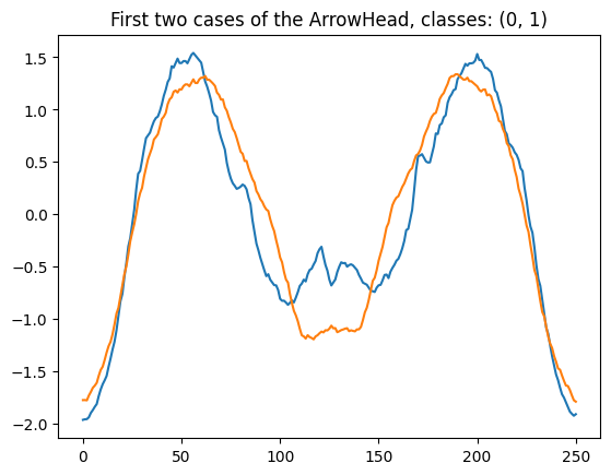
The arrowhead data consists of outlines of the images of arrowheads. The shapes of the projectile points are converted into a time series using the angle-based method. The classification of projectile points is is an important topic in anthropology. The classes are based on shape distinctions, such as the presence and location of a notch in the arrow. The problem in the repository is a length normalised version of that used in Ye09shapelets. The three classes are called “Avonlea” (0), “Clovis” (1) and “Mix” (2).

from aeon.datasets import load_arrow_head

arrowhead, arrow_labels = load_arrow_head()
print(arrowhead.shape)
plt.title(
    f"First two cases of the ArrowHead, classes: "
    f"({arrow_labels[0]}, {arrow_labels[1]})"
)

plt.plot(arrowhead[0][0])
plt.plot(arrowhead[1][0])

(211, 1, 251)

[<matplotlib.lines.Line2D at 0x159d38626d0>]

BasicMotions

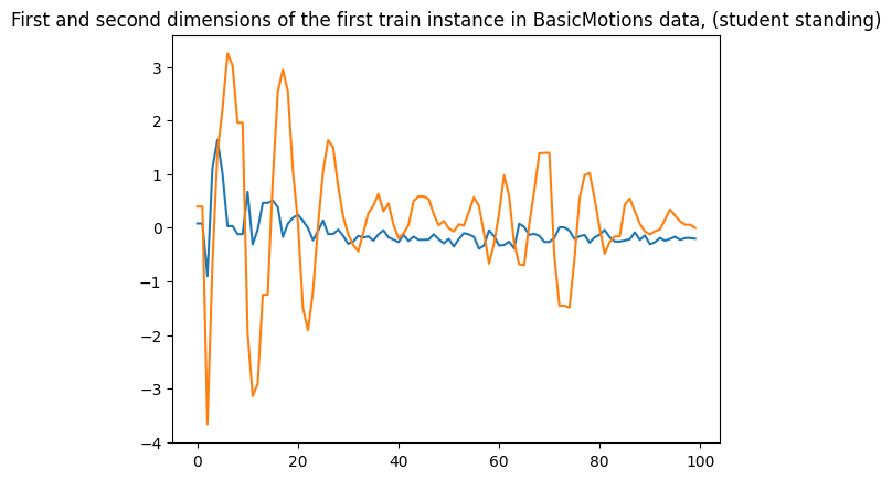
The data was generated as part of a student project where four students performed our activities whilst wearing a smart watch. The watch collects 3D accelerometer and a 3D gyroscope It consists of four classes, which are walking, resting, running and badminton. Participants were required to record motion a total of five times, and the data is sampled once every tenth of a second, for a ten second period. The data is multivariate (six channels) equal length.

from aeon.datasets import load_basic_motions

motions, motions_labels = load_basic_motions(split="train")
plt.title(
    f"First and second dimensions of the first train instance in BasicMotions data, "
    f"(student {motions_labels[0]})"
)
plt.plot(motions[0][0])
plt.plot(motions[0][1])

[<matplotlib.lines.Line2D at 0x159d589ffa0>]

GunPoint

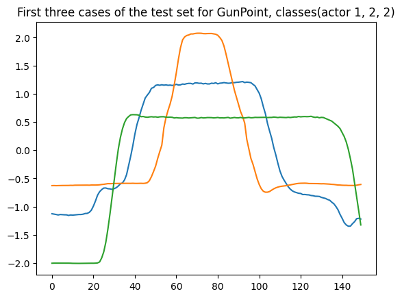
This dataset involves one female actor and one male actor making a motion with their hand. The two classes are: Gun-Draw and Point: For Gun-Draw the actors have their hands by their sides. They draw a replicate gun from a hip-mounted holster, point it at a target for approximately one second, then return the gun to the holster, and their hands to their sides. For Point the actors have their gun by their sides. They point with their index fingers to a target for approximately one second, and then return their hands to their sides. For both classes, The data in the archive is the X-axis motion of the actors right hand.

from aeon.datasets import load_gunpoint

gun, gun_labels = load_gunpoint(split="test")
plt.title(
    f"First three cases of the test set for GunPoint, classes"
    f"(actor {gun_labels[0]}, {gun_labels[1]}, {gun_labels[2]})"
)
plt.plot(gun[0][0])
plt.plot(gun[1][0])
plt.plot(gun[2][0])

[<matplotlib.lines.Line2D at 0x159d62fc5e0>]

ItalyPowerDemand

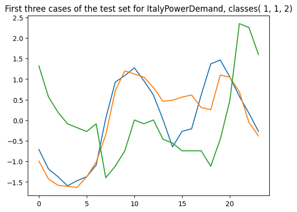
The data was derived from twelve monthly electrical power demand time series from Italy and first used in the paper “Intelligent Icons: Integrating Lite-Weight Data Mining and Visualization into GUI Operating Systems”. The classification task is to distinguish days from Oct to March (inclusive) (class 0) from April to September (class 1). The problem is univariate, equal length.

from aeon.datasets import load_italy_power_demand

italy, italy_labels = load_italy_power_demand(split="train")
plt.title(
    f"First three cases of the test set for ItalyPowerDemand, classes"
    f"( {italy_labels[0]}, {italy_labels[1]}, {italy_labels[2]})"
)
plt.plot(italy[0][0])
plt.plot(italy[1][0])
plt.plot(italy[2][0])

[<matplotlib.lines.Line2D at 0x159d6350670>]

JapaneseVowels

A UCI Archive dataset. See this link for more detailed information

Paper: M. Kudo, J. Toyama and M. Shimbo. (1999). “Multidimensional Curve Classification Using Passing-Through Regions”. Pattern Recognition Letters, Vol. 20, No. 11–13, pages 1103–1111.

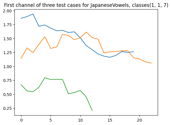
9 Japanese-male speakers were recorded saying the vowels ‘a’ and ‘e’. A ‘12-degree linear prediction analysis’ is applied to the raw recordings to obtain time-series with 12 dimensions and series lengths between 7 and 29. The classification task is to predict the speaker. Therefore, each instance is a transformed utterance, 12*29 values with a single class label attached, [1…9].

The given training set is comprised of 30 utterances for each speaker, however the test set has a varied distribution based on external factors of timing and experimental availability, between 24 and 88 instances per speaker. The data is unequal length

from aeon.datasets import load_japanese_vowels

japan, japan_labels = load_japanese_vowels(split="train")
plt.title(
    f"First channel of three test cases for JapaneseVowels, classes"
    f"({japan_labels[0]}, {japan_labels[10]}, {japan_labels[200]})"
)
print(f" number of cases = " f"{len(japan)}")
print(f" First case shape = " f"{japan[0].shape}")
print(f" Tenth case shape = " f"{japan[10].shape}")
print(f" 200th case shape = " f"{japan[200].shape}")

plt.plot(japan[0][0])
plt.plot(japan[10][0])
plt.plot(japan[200][0])

 number of cases = 270
 First case shape = (12, 20)
 Tenth case shape = (12, 23)
 200th case shape = (12, 13)

[<matplotlib.lines.Line2D at 0x159d63d5c40>]

OSUleaf

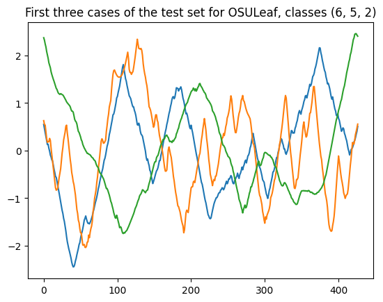
The OSULeaf data set consist of one dimensional outlines of leaves. The series were obtained by color image segmentation and boundary extraction (in the anti-clockwise direction) from digitized leaf images of six classes: Acer Circinatum, Acer Glabrum, Acer Macrophyllum, Acer Negundo, Quercus Garryana and Quercus Kelloggii for the MSc thesis “Content-Based Image Retrieval: Plant Species Identification” by A. Grandhi. OSULeaf is equal length and univariate

from aeon.datasets import load_osuleaf

leaf, leaf_labels = load_osuleaf(split="train")
plt.title(
    f"First three cases of the test set for OSULeaf, classes"
    f" ({leaf_labels[0]}, {leaf_labels[1]}, {leaf_labels[2]})"
)
plt.plot(leaf[0][0])
plt.plot(leaf[1][0])
plt.plot(leaf[2][0])

[<matplotlib.lines.Line2D at 0x159d6454c40>]

PLAID

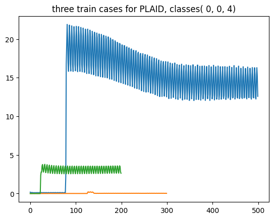
PLAID stands for the Plug Load Appliance Identification Dataset. The data are intended for load identification research. The first version of PLAID is named PLAID1, collected in summer 2013. A second version of PLAID was collected in winter 2014 and released under the name PLAID2. This dataset comes from PLAID1. It includes current and voltage measurements sampled at 30 kHz from 11 different appliance types present in more than 56 households in Pittsburgh, Pennsylvania, USA. Data collection took place during the summer of 2013. Each appliance type is represented by dozens of different instances of varying makes/models. For each appliance, three to six measurements were collected for each state transition. These measurements were then post-processed to extract a few-second-long window containing both the steady-state operation and the startup transient )when available). The classes correspond to 11 different appliance types: air conditioner (class 0), compact flourescent lamp, fan, fridge, hairdryer , heater, incandescent light bulb, laptop, microwave, vacuum,washing machine (class 10). The data is univariate and unequal length.

from aeon.datasets import load_plaid

plaid, plaid_labels = load_plaid(split="train")
plt.title(
    f"three train cases for PLAID, classes"
    f"( {plaid_labels[0]}, {plaid_labels[10]}, {plaid_labels[200]})"
)
print(f" number of cases = " f"{len(plaid)}")
print(f" First case shape = " f"{plaid[0].shape}")
print(f" Tenth case shape = " f"{plaid[10].shape}")
print(f" 200th case shape = " f"{plaid[200].shape}")

plt.plot(plaid[0][0])
plt.plot(plaid[10][0])
plt.plot(plaid[200][0])

 number of cases = 537
 First case shape = (1, 500)
 Tenth case shape = (1, 300)
 200th case shape = (1, 200)

[<matplotlib.lines.Line2D at 0x159d651e7f0>]

Regression

We ship one regression problem from the [Time Series Extrinsic Regression] (http://tseregression.org/) website and one soon to be added.

Covid3Month

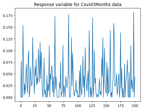
The goal of this dataset is to predict COVID-19’s death rate on 1st April 2020 for each country using daily confirmed cases for the last three months. This dataset contains 201 time series, where each time series is the daily confirmed cases for a country. The data was obtained from WHO’s COVID-19 database. Please refer to https://covid19.who.int/ for more details

from aeon.datasets import load_covid_3month

covid, covid_target = load_covid_3month()
print(covid.shape)
plt.title("Response variable for Covid3Months data")
plt.plot(covid_target)

(201, 1, 84)

[<matplotlib.lines.Line2D at 0x159d6591820>]

CardanoSentiment

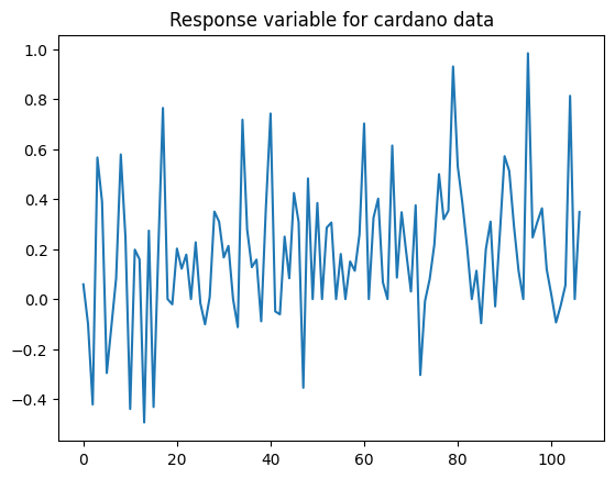
By combining historical sentiment data for Cardano cryptocurrency, extracted from EODHistoricalData and made available on Kaggle, with historical price data for the same cryptocurrency, extracted from CryptoDataDownload, we created the CardanoSentiment dataset, with 107 instances. The predictors are hourly close price (in USD) and traded volume during a day, resulting in 2-dimensional time series of length 24. The response variable is the normalized sentiment score on the day spanned by the timepoints.

from aeon.datasets import load_cardano_sentiment

cardano, cardano_target = load_cardano_sentiment()
print(cardano.shape)
plt.title("Response variable for cardano data")
plt.plot(cardano_target)

(107, 2, 24)

[<matplotlib.lines.Line2D at 0x159d630f8e0>]

Segmentation

Two of the UCR classification data have been adapted for segmentation.

ElectricDevices

The UCR ElectricDevices dataset series are grouped by class label and concatenated to create segments with repeating temporal patterns and characteristics. The location at which different classes were concatenated are marked as change points.

this function returns a single series, the period length as an integer and the change points as a numpy array.

from aeon.datasets import load_electric_devices_segmentation

data, period, change_points = load_electric_devices_segmentation()
print(" Period = ", period)
print(" Change points = ", change_points)
plot_series(data)

 Period =  10
 Change points =  [1090 4436 5712 7923]

(<Figure size 1600x400 with 1 Axes>, <Axes: ylabel='1'>)

GunPoint Segmentation

The UCR GunPoint dataset series are grouped by class label and concatenated to create segments with repeating temporal patterns and characteristics. The location at which different classes were concatenated are marked as change points.

this function returns a single series, the period length as an integer and the change points as a numpy array.

from aeon.datasets import load_gun_point_segmentation

data, period, change_points = load_gun_point_segmentation()
print(" Period = ", period)
print(" Change points = ", change_points)
plot_series(data)

 Period =  10
 Change points =  [900]

(<Figure size 1600x400 with 1 Axes>, <Axes: ylabel='1'>)

---

Generated using nbsphinx. The Jupyter notebook can be found here.