The Signature Method with aeon

The ‘signature method’ refers to a collection of feature extraction techniques for multimodal sequential data, derived from the theory of controlled differential equations. In recent years, a large number of modifications have been suggested to the signature method so as to improve some aspect of it.

In the paper “A Generalised Signature Method for Time-Series” [1] the authors collated the vast majority of these modifications into a single document and ran a large hyper-parameter study over the multivariate UEA datasets to build a generic signature algorithm that is expected to work well on a wide range of datasets. We implement the best practice results from this study as the default starting values for our hyperparameters in the SignatureClassifier module.

The Path Signature

At the heart of the signature method is the so-called “signature transform”.

A path \(X\) of finite length in \(\textit{d}\) dimensions can be described by the mapping \(X:[a, b]\rightarrow\mathbb{R}\) \(\!\!^d\), or in terms of co-ordinates \(X=(X^1_t, X^2_t, ...,X^d_t)\), where each coordinate \(X^i_t\) is real-valued and parameterised by \(t\in[a,b]\).

The signature transform \(S\) of a path \(X\) is defined as an infinite sequence of values:

:nbsphinx-math:`begin{equation}

S(X)_{a, b} = (1, S(X)_{a, b}^1, S(X)_{a, b}^2, …, S(X)_{a, b}^d, S(X)_{a,b}^{1, 1}, S(X)_{a,b}^{1, 2}, …), label{eq:path_signature}

end{equation}` where each term is a \(k\)-fold iterated integral of \(X\) with multi-index \(i_1,...,i_k\): :nbsphinx-math:`begin{equation}

S(X)_{a, b}^{i_1,…,i_k} = int_{a<t_k<b}…int_{a<t_1<t_2} mathrm{d}X_{t_1}^{i_1}…mathrm{d}X_{t_k}^{i_k}. label{eq:sig_moments}

end{equation}` This defines a graded sequence of numbers associated with a path which is known to characterise it up to a generalised form of reparameterisation [2]. One can think of the signature as a collection of summary statistics that determine a path (almost) uniquely. Furthermore, any continuous function on the path \(X\) can be approximated arbitrarily well as a linear function on its signature [3]; the signature unravels the non-linearities on functions on the space of unparameterised paths.

A Visualisation

To give an idea of what the signature terms represent physically, we consider a patient in an ICU where we are tracking their systolic blood pressure (SBP) and heart rate (HR) changing in time. This can be represented as a path in \(\mathbb{R}^3\) (assuming time is included as a channel).

signature_visualisation

The plot above sketches two scenarios of how such a path might look. We are assuming here an implicit time dimension for each plot such that the path is traversed from left to right along the blue line.

Depth 1:

The signature terms to depth 1 are simply the changes of each of the variables over the interval, in the image this is the \(\Delta \text{HR}\) and \(\Delta \text{SBP}\) terms. Note that these values are the same in each case.

Depth 2:

The second level gives us the signed areas (the shaded orange regions), where the orientation of the left most plot is such that the negatively signed area is produced whereas the second gives the positive value, and thus, at order 2 in the signature we now have sufficient information to discriminate between these two situations where in the first rise in heart rate occurs before (or at least, initially faster than) the rise in blood pressure, and vice versa.

Depth > 2:

Depths larger than 2 become more difficult to visualise graphically, however the idea is similar to that of the depth 2 case where we saw that the signature produced information on whther the increase in HR or SBP appeared to be happening first, along with some numerical quantification of how much this was happening. At higher orders the signature is doing something similar, but now with three events, rather than two. The signature picks out structural information regarding the order in which events occur.

The Signature in Time-Series Analysis

The signature is a natural tool to apply in problems related to time-series analysis. As described above it can convert multi-dimensional time-series data into static features that represent information about the sequential nature of the time-series, that can be fed through a standard machine learning model.

A simplistic view of how this works is as follows: :nbsphinx-math:`begin{equation}

text{Model}(text{Signature}(text{Sequential data}))) = text{Predictions}

end{equation}`

Considered Signature Variations

Again, following the work in [1] we group the variations on the siganture method conceptually into:

• Augmentations - Transformation of an input sequence or time series into one or more new sequences, so that the signature will return different information about the path.

• Windows - Windowing operations, so that the signature can act with some locality.

• Transforms - The choice between the signature or the logsignature transformation.

• Rescalings - Method of signature rescaling.

This is neatly represented in the following graphic, where \(\phi\) represents the augmentation, \(W^{i, j}\) the windowing operation, \(S^N\) the signature, and \(\rho_{\text{pre}/\text{post}}\) the rescaling method.

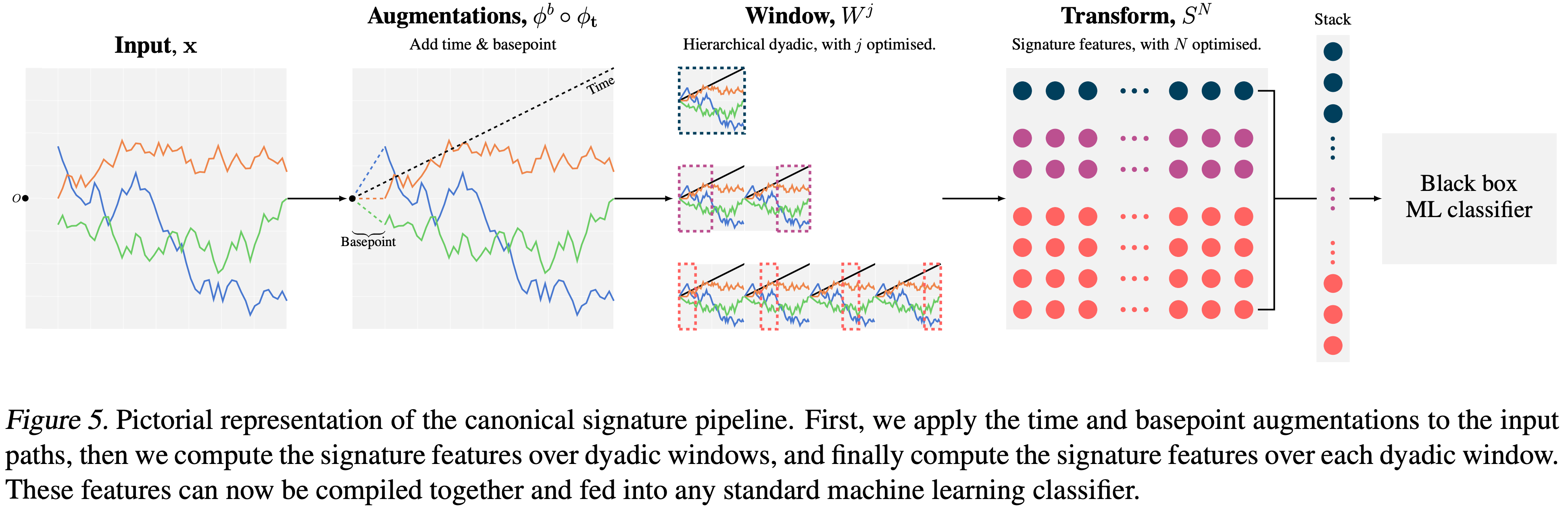
Please refer to the full paper for a more comprehensive exploration into what each of these groupings means.

The aeon Modules

We now give an introduction to the classification and transformation modules included in th aeon interface, along with an example to show how to perform efficient hyperparameter optimisation that was found to give good results in [1].

# Some additional imports we will use
from sklearn.ensemble import RandomForestClassifier
from sklearn.metrics import accuracy_score

from aeon.datasets import load_unit_test

# Load an example dataset
train_x, train_y = load_unit_test(split="train")
test_x, test_y = load_unit_test(split="test")

Overview

We provide the following: - aeon.transformers.panel.signature_based.SignatureTransformer - An sklearn transformer that provides the functionality to apply the signature method with some choice of variations as noted above. - aeon.classification.feature_based.SignatureClassifier - This provides a simple interface to append a classifier to the SignatureTransformer class.

from aeon.classification.feature_based import SignatureClassifier
from aeon.transformations.collection.signature_based import SignatureTransformer

Example 1: Sequential Data -> Signature Features.

Here we will give a very simple example of converting the sequential 3D GunPoint data of shape [num_batch, n_timepoints, num_features] -> [num_batch, signature_features].

# First build a very simple signature transform module
signature_transform = SignatureTransformer(
    augmentation_list=("addtime",),
    window_name="global",
    window_depth=None,
    window_length=None,
    window_step=None,
    rescaling=None,
    sig_tfm="signature",
    depth=3,
)

# The simply transform the stream data
print("Raw data shape is: {}".format(train_x.shape))
train_signature_x = signature_transform.fit_transform(train_x)
print("Signature shape is: {}".format(train_signature_x.shape))

Raw data shape is: (20, 1, 24)
Signature shape is: (20, 14)

It then becomes easy to build a time-series classification model. For example:

# Train
model = RandomForestClassifier()
model.fit(train_signature_x, train_y)

# Evaluate
test_signature_x = signature_transform.transform(test_x)
test_pred = model.predict(test_signature_x)
print("Accuracy: {:.3f}%".format(accuracy_score(test_y, test_pred)))

Accuracy: 0.864%

Example 2: Fine Tuning the Generalised Model

As previously mentioned, in [1] the authors performed a large hyperparameter search over the signature variations on the full UEA archive to develop a ‘Best Practices’ approach to building a model. This required some fine tuning over the following parameters, as they were found to be very dataset specific: - depth over [1, 2, 3, 4, 5, 6] - window_depth over [2, 3, 4] - RandomForestClassifier hyperparamters.

Here we show a simplified version of the tuning.

from sklearn.model_selection import RandomizedSearchCV, StratifiedKFold

# Some params
n_cv_splits = 5
n_gs_iter = 5

# Random forests found to perform very well in general
estimator = RandomForestClassifier()

# The grid to be passed to an sklearn gridsearch
signature_grid = {
    # Signature params
    "depth": [1, 2],
    "window_name": ["dyadic"],
    "augmentation_list": [["basepoint", "addtime"]],
    "window_depth": [1, 2],
    "rescaling": ["post"],
    # Classifier and classifier params
    "estimator": [estimator],
    "estimator__n_estimators": [50, 100],
    "estimator__max_depth": [2, 4],
}

# Initialise the estimator
estimator = SignatureClassifier()

# Run a random grid search and return the gs object
cv = StratifiedKFold(n_splits=n_cv_splits)
gs = RandomizedSearchCV(estimator, signature_grid, cv=n_cv_splits, n_iter=n_gs_iter)
gs.fit(train_x, train_y)

# Get the best classifier
best_classifier = gs.best_estimator_

# Evaluate
train_preds = best_classifier.predict(train_x)
test_preds = best_classifier.predict(test_x)
train_score = accuracy_score(train_y, train_preds)
test_score = accuracy_score(test_y, test_preds)
print(
    "Train acc: {:.3f}%  |  Test acc: {:.3f}%".format(
        train_score * 100, test_score * 100
    )
)

C:\Code\aeon\venv\lib\site-packages\sklearn\model_selection\_search.py:305: UserWarning: The total space of parameters 16 is smaller than n_iter=20. Running 16 iterations. For exhaustive searches, use GridSearchCV.
  warnings.warn(

Train acc: 100.000%  |  Test acc: 95.455%

A Full Description of the Parameters

We conclude by giving further explanation of each of the parameters in the SignatureClassifier module and what values they can take.

Parameters

Below we list each parameter and the values that they can take. For further details about what the options mean refer to [1].

classifier Needs to be any sklearn estimator. Defaults to RandomForestClassifier().

augmentation_list: list of tuple of strings, List of augmentations to be applied before the signature transform is applied. These can be any from: - ‘addtime’ - Add an equally spaced time channel. - ‘leadlag’ - The leadlag transform. - ‘ir’ - Perform the invisibility reset transform. - ‘cumsum’ - Perform a cumulative sum transform. - ‘basepoint’ - Append zero to the start of the path to remove translational invariance.

window_name str, The name of the window transform to apply. Can be any of: - ‘global’ - A single window over all the data. - ‘expanding’ - Multiple windows starting at the first datapoint that extend over the data (increasing width). - ‘sliding’ - Multiple windows that slide along the data (fixed width). - ‘dyadic’ - Partition the data into dyadic windows.

window_depth: int, The depth of the dyadic window. (Active only if window_name == 'dyadic']).

window_length: int, The length of the sliding/expanding window. (Active only if window_name in ['sliding, 'expanding'].)

window_step: int, The step of the sliding/expanding window. (Active only if window_name in ['sliding, 'expanding'].)

rescaling: str, The method of signature rescaling. Any of: - ‘pre’ - Rescale the path before the signature transform. - ‘post’ - Rescale the path after the signature transform. - None - No rescaling.

sig_tfm: str, String to specify the type of signature transform. Either of: [‘signature’, ‘logsignature’].

depth: int, Signature truncation depth.

random_state: int, Random state initialisation.

References

[1] Morrill, James, Adeline Fermanian, Patrick Kidger, and Terry Lyons. “A Generalised Signature Method for Time Series.” arXiv preprint arXiv:2006.00873 (2020).

[2] Hambly, B., Lyons, T.: Uniqueness for the signature of a path of bounded variation and the reduced pathgroup. Annals of Mathematics171(1), 109–167 (2010). doi:10.4007/annals.2010.171.10913.

[3] Lyons, T.J.: Differential equations driven by rough signals. Revista Matem ́atica Iberoamericana14(2), 215–310(1998)

---

Generated using nbsphinx. The Jupyter notebook can be found here.