Distance Functions in aeon

Measuring the distance or similarity between time series is a key primitive operation in a range of time series machine learning tasks. This notebook describes the core distance functionality available in aeon, focusing on two key distance measures, Euclidean distance and dynamic time warping. We describe the full range of distance functions available in [1] and show how they can be used with aeon and scikit-learn estimators on this page.

The goal of a distance computation is to measure the dis-similarity between the time series a and b. A distance function should take a and b as parameters and return a float that is the computed distance between a and b. The value returned should be 0.0 when the time series are exactly the same, and, when they are different, a value greater than 0.0 that is a measure of distance between them.

Distance functions can be used in all time series machine learning tasks. In classification and regression they are employed in, for example nearest neighbour classifiers/regressors. In clustering they are central to \(k\)-means and \(k\)-medoids clustering.

This notebook provides a simple use case for distances and motivates why we need elastic distances. It introduces the most popular elastic distance measure, dynamic time warping, and describes how it is used and parameterised in aeon. We show how to retrieve all pairwise distances for a collection of series and how to use distances with multivariate time series distances. Distances can be used to find alignment paths, and with unequal length series.

Simple use case for distances

distance functions take two 1D or 2D numpy array input and calculate a distance. If a series has more than one channel (i.e. multivariate time series), it should be stored as shape (d,n). Univariate time series of length \(n\) can be modelled as either shape (n,) or (1,n). The simplest distance is Euclidean distance. This measures the sum of squared distances between points.

\[d_e(a, b) = \sqrt{\sum_{i=1}^m(a_i-b_i)}\]

The most popular time series specific distance is dynamic time warping (DTW). These and other distance functions are imported form aeon.distances.

import warnings

import numpy as np

from aeon.distances import dtw_distance, euclidean_distance

warnings.filterwarnings("ignore")
a = np.array([1, 2, 3, 4, 5, 6])  # Univariate as 1D
b = np.array([2, 3, 4, 5, 6, 7])
d1 = euclidean_distance(a, b)
d2 = dtw_distance(a, b)
print(f" ED 1 = {d1} DTW 1 = {d2}")
x = np.array([[1, 2, 3, 4, 5, 6]])  # Univariate as 2D
y = np.array([[2, 3, 4, 5, 6, 7]])
d1 = euclidean_distance(x, y)
d2 = dtw_distance(x, y)
print(f" ED 2 = {d1} DTW 2 = {d2}")
x = np.array([[1, 2, 3, 4, 5, 6], [3, 4, 3, 4, 3, 4]])  # Multivariate, 2 channels
y = np.array([[2, 3, 4, 5, 6, 7], [7, 6, 5, 4, 3, 2]])
d1 = euclidean_distance(x, y)
d2 = dtw_distance(x, y)
print(f" ED 3 = {d1} DTW 3 = {d2}")

 ED 1 = 2.449489742783178 DTW 1 = 2.0
 ED 2 = 2.449489742783178 DTW 2 = 2.0
 ED 3 = 5.830951894845301 DTW 3 = 34.0

Basic Motivation for Elastic Distances

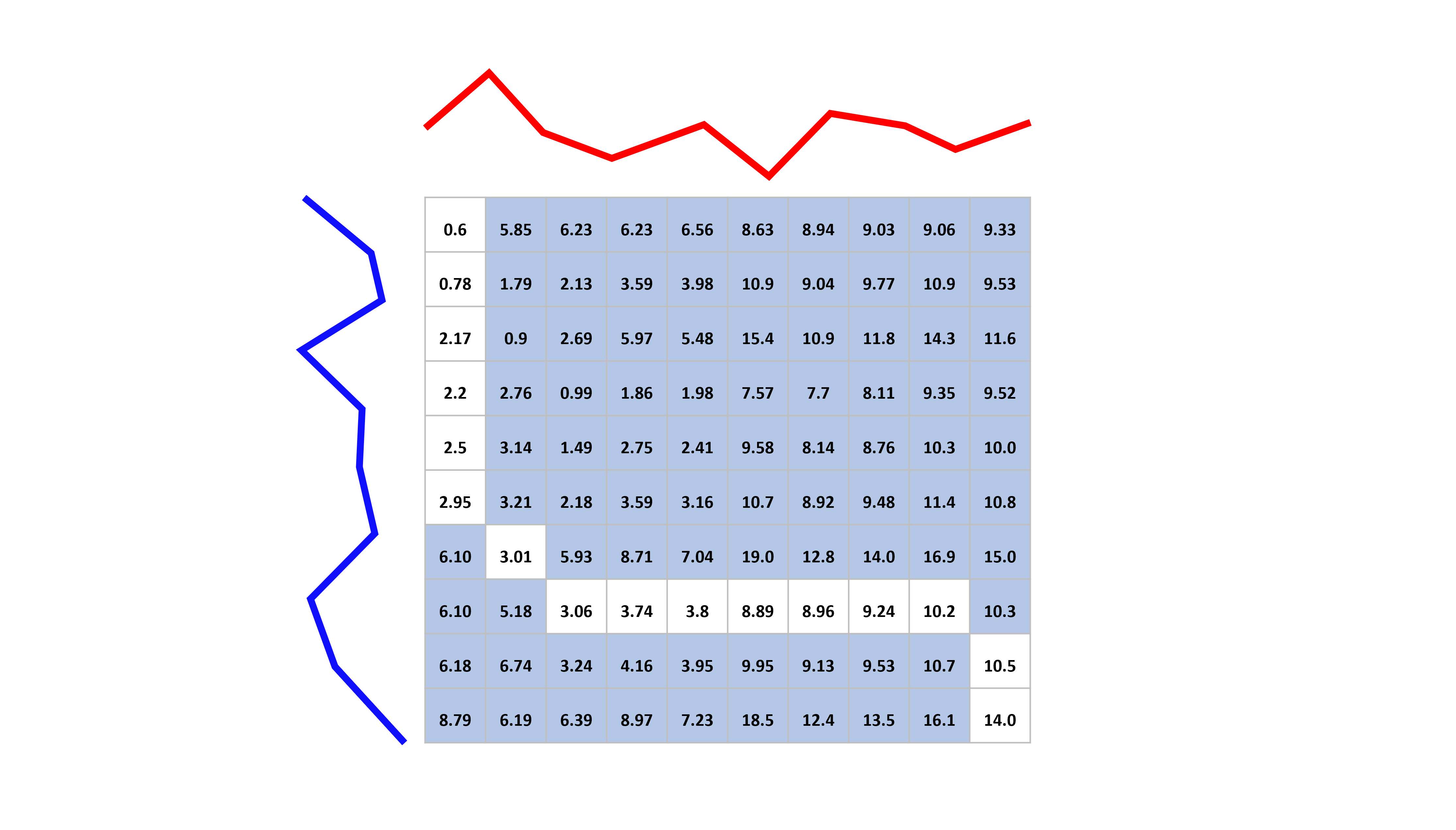
As an example we will use data from the gunpoint data. This is a two class problem. If a distance function is to be useful, we hope it will measure lower distances between instances of the same class than those of different classes. We extract three cases as an example.

import matplotlib.pyplot as plt
import numpy as np

from aeon.datasets import load_gunpoint

X, y = load_gunpoint()
print(X.shape)
first = X[1][0]
second = X[2][0]
third = X[4][0]
plt.plot(first, label="First series")
plt.plot(second, label="Second series")
plt.plot(third, label="Third series")
plt.legend()
print(f" class values {y[1]}, {y[2]}, {y[4]}")

(200, 1, 150)
 class values 2, 1, 2

The problem with Euclidean distance is it takes no account of the order, and so a small offset can lead to large distances. For this problem, the discriminatory information is in the small areas before and after the peak (around points 30-50 and 100-130). In the example above, the first and third example are in the same class, but the peaks are offset. This means there is a larger distance between these cases and the second example. Note that you can also find distances by calling distance with a string parameter for the distance like so:

from aeon.distances import distance, euclidean_distance

d1 = euclidean_distance(first, second)
d2 = euclidean_distance(first, third)
d3 = distance(second, third, metric="euclidean")
print(d1, ",", d2, ",", d3)

2.490586847171778 , 6.307592298519925 , 6.618889405616554

Elastic distances such dynamic time warping realign series to compensate for offset. If we use dtw_distance instead of euclidean_distance

from aeon.distances import dtw_distance

d1 = dtw_distance(first, second)
d2 = dtw_distance(first, third)
d3 = dtw_distance(second, third)
print(d1, ",", d2, ",", d3)

1.733128174164524 , 0.5299968542651227 , 3.666430398991013

we see now the first example is closer to the one in its own class than the second example.

Dynamic time warping

Dynamic time warping (DTW) [2] is an elastic distance measure that works by first calculating all the (\(m,m\) square pointwise distance matrix \(M\) between all points in the series, $ M_{i,j}(a,b) = (a_i-b_j)^2 $ then using \(M\) to find the minimum path through this matrix to minimise the total cost of traversal, allowing movement forward of one square at a time. For following algorithm includes a bounding matrix (see below).

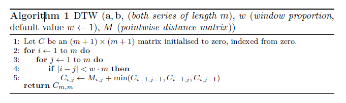
The warping path can be seen as the path of least resistance through the cost matrix C found throug a dynamic programming formulation.

Custom parameters for distances

Each distance function has a different set of parameters. For specific parameters for each distance please refer to the documentation.

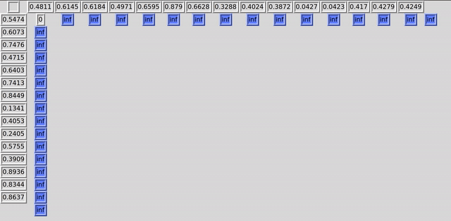
DTW is a \(O(n^2)\) algorithm and as such a point of focus has been trying to optimise the algorithm. A proposal to improve performance is to restrict the potential alignment path by putting a ‘bound’ on values to consider when looking for an alignment. While there have been many bounding algorithms proposed the most popular is known as Sakoe-Chiba’s bounding window.

This is implemented in aeon using a bounding box mask, where False indicates an invalid move. The bounding matrix that considers all indexes in a and b:

from aeon.distances import create_bounding_matrix

first_ts_size = 10
second_ts_size = 10

create_bounding_matrix(first_ts_size, second_ts_size)

array([[ True,  True,  True,  True,  True,  True,  True,  True,  True,
         True],
       [ True,  True,  True,  True,  True,  True,  True,  True,  True,
         True],
       [ True,  True,  True,  True,  True,  True,  True,  True,  True,
         True],
       [ True,  True,  True,  True,  True,  True,  True,  True,  True,
         True],
       [ True,  True,  True,  True,  True,  True,  True,  True,  True,
         True],
       [ True,  True,  True,  True,  True,  True,  True,  True,  True,
         True],
       [ True,  True,  True,  True,  True,  True,  True,  True,  True,
         True],
       [ True,  True,  True,  True,  True,  True,  True,  True,  True,
         True],
       [ True,  True,  True,  True,  True,  True,  True,  True,  True,
         True],
       [ True,  True,  True,  True,  True,  True,  True,  True,  True,
         True]])

Above shows a matrix that maps each index in ‘a’ to each index in ‘b’. Each value that is considered in the computation is set to True (in this instance we want a full bounding matrix so all values are set to True). This means we can warp any index onto another.

However, it sometimes (depending on the dataset) is not necessary (and sometimes detrimental to the result) to consider all indexes. We can use a bounding technique like Sakoe-Chibas to limit the potential warping paths. This is done by setting a window size that will restrict the indexes that are considered. Below shows creating a bounding matrix again but only considering 20% of the indexes in x and y:

create_bounding_matrix(first_ts_size, second_ts_size, window=0.2)

array([[ True,  True,  True, False, False, False, False, False, False,
        False],
       [ True,  True,  True,  True, False, False, False, False, False,
        False],
       [ True,  True,  True,  True,  True, False, False, False, False,
        False],
       [False,  True,  True,  True,  True,  True, False, False, False,
        False],
       [False, False,  True,  True,  True,  True,  True, False, False,
        False],
       [False, False, False,  True,  True,  True,  True,  True, False,
        False],
       [False, False, False, False,  True,  True,  True,  True,  True,
        False],
       [False, False, False, False, False,  True,  True,  True,  True,
         True],
       [False, False, False, False, False, False,  True,  True,  True,
         True],
       [False, False, False, False, False, False, False,  True,  True,
         True]])

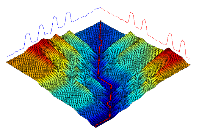
This bounding matrix produces a corridor of allowed warping. A nice visualisation of DTW with a constained window from https://github.com/hadifawaz1999/DTW_GUI

From a users perspective, the easiest way to constrain DTW with a bounding window is to set the parameter window, which sets the maximum percentage of series length of warping allowed. No window (window=0.0) corresponds to the squared Euclidean distance. The default value is full window (window=1.0) which means full warping. A common default setting is to use window=0.2 and this is often referred to as constrained DTW (cdtw).

Note that we do not take the square root of DTW, because it is not necessary for any of the applications used in aeon, which require ordering time series by distances.

a = np.array([1, 3, 4, 5, 7, 10, 3, 2, 1])
b = np.array([1, 4, 5, 7, 10, 3, 2, 1, 1])
c = np.array([1, 2, 5, 5, 5, 5, 5, 2, 1])
plt.plot(a, label="Series a")
plt.plot(b, label="Series b")
plt.plot(c, label="Series c")
plt.legend()
d1 = euclidean_distance(a, b)
d2 = euclidean_distance(a, c)
print("Euclidean distance a to b =", d1)
print("Euclidean distance a to c =", d2)
d1 = dtw_distance(a, b, window=0.0)
d2 = dtw_distance(a, b, window=1.0)
d3 = dtw_distance(a, b, window=0.2)
d4 = euclidean_distance(a, b) ** 2
print("Zero window DTW distance (Squared Euclidean) from a to b =", d1)
print("Squared Euclidean = ", d4)
print("DTW distance (full window) a to b =", d2)
print("DTW distance (20% warping window) a to b =", d3)

Euclidean distance a to b = 8.12403840463596
Euclidean distance a to c = 5.916079783099616
Zero window DTW distance (Squared Euclidean) from a to b = 66.0
Squared Euclidean =  66.00000000000001
DTW distance (full window) a to b = 1.0
DTW distance (20% warping window) a to b = 1.0

Pairwise distances

It is common to want a matrix of pairwise distances for a collation of time series. For example, medoid based clustering and certain sklearn estimators can work directly with precalculated distance matrices rather than repeated calls to a distance function. It is easy to get a distance matrix from a pairwise distance function in aeon. This can either be for a single collection or for two collections. This is useful with sklearn. We use MSM distance in this example simply for variety.

from aeon.datasets import load_arrow_head
from aeon.distances import msm_pairwise_distance

X_train, _ = load_arrow_head(split="train")
X_test, _ = load_arrow_head(split="test")
X1 = X_train[:5]
X2 = X_test[:6]
train_dist_matrix = msm_pairwise_distance(X1)
test_dist_matrix = msm_pairwise_distance(X1, X2)
print(
    f"Single X dist pairwise is square and symmetrical shape "
    f"= {train_dist_matrix.shape}\n{train_dist_matrix}"
)
print(
    f"Two X dist pairwise is all dists from X1 (row) to X2 (column), so shape "
    f"shape = {test_dist_matrix.shape}\n{test_dist_matrix}"
)

Single X dist pairwise is square and symmetrical shape = (5, 5)
[[ 0.         62.2553732  45.91702356 49.72138985 50.07185968]
 [62.2553732   0.         31.06762179 93.31791099 25.73406576]
 [45.91702356 31.06762179  0.         82.05754675 32.71868983]
 [49.72138985 93.31791099 82.05754675  0.         79.50156797]
 [50.07185968 25.73406576 32.71868983 79.50156797  0.        ]]
Two X dist pairwise is all dists from X1 (row) to X2 (column), so shape shape = (5, 6)
[[ 21.01701605  22.16699488  86.45534374  75.69573009  48.79410225
   33.27495124]
 [ 63.76668286  59.61188967  93.89293437 109.6967054   92.68370785
   47.78485799]
 [ 44.01308016  39.55587095  99.06160623  94.98620404  85.33606252
   34.36027177]
 [ 53.21801989  60.05103978  72.37115291  64.11310795  24.86221373
   66.65632674]
 [ 48.70558166  48.82369739  88.5358956  101.44412148  80.20208926
   37.59557677]]

Alignment paths

When elastic distances are calculated, they effectively align the two indexes. You can directly recover the warping path (or alignment paths) using provided functions.

from aeon.distances import alignment_path, dtw_alignment_path

x = np.array([[1, 2, 3, 4, 5, 6]])  # Univariate as 2D
y = np.array([[2, 3, 4, 5, 6, 7]])
p, d = dtw_alignment_path(x, y)
print("path =", p, " distance = ", d)
p, d = alignment_path(x, y, metric="dtw")
print("path =", p, " distance = ", d)

path = [(0, 0), (1, 0), (2, 1), (3, 2), (4, 3), (5, 4), (5, 5)]  distance =  2.0
path = [(0, 0), (1, 0), (2, 1), (3, 2), (4, 3), (5, 4), (5, 5)]  distance =  2.0

Multivariate distances

aeon models a single multivariate time series as 2D numpy arrays of shape (n_channels, n_timepoints). Note we only support multivariate instances where each channel is the same length, and we assume they are aligned. Basic motions is a data set recording the (x,y,z) trace of motions taken from a smart watch

from aeon.datasets import load_basic_motions

motions, _ = load_basic_motions()
plt.plot(motions[0][0], label="First channel")
plt.plot(motions[0][1], label="Second channel")
plt.plot(motions[0][2], label="Third channel")
plt.legend()

<matplotlib.legend.Legend at 0x16f8ae3c8e0>

Suppose we have \(k\) channels in our multivariate time series. There are two ways to find the distance between two time series \(a\) and \(b\) of shape \((c,m)\).

1. Independent: we find the distance between each channel independently, then sum them to get the final distance. So if we are using univariate distance \(d\), the multivariate version is

   \[d_m(a,b) = \sum_{c=1}^k d(a_c, b_c)\]

2. Dependent: We use all channels during the calculation of the pointwise distance matrix \(M\), so that

   \[M_{i,j}(a,b) = \sum_{c=1}^k (a_{c,i}-b_{c,j})^2\]

   The distance then is calculated as before using this version of \(M\).

aeon assumes the dependent approach. It is simple to get an independent version by iterating over dimensions.

d1 = dtw_distance(motions[0], motions[1])
print("Dependent DTW distance (multivariate) motions[0] to motions[1] =", d1)
s = 0
for k in range(motions[0].shape[0]):
    s += dtw_distance(motions[0][k], motions[1][k])
print("Independent DTW distance (multivariate) motions[0] to motions[1] =", s)

Dependent DTW distance (multivariate) motions[0] to motions[1] = 330.83449721446283
Independent DTW distance (multivariate) motions[0] to motions[1] = 219.03725136740098

Unequal length series

Distance functions work with unequal length series, although a multivariate series must have the same length for each channel (numpy does not allow ragged arrays)

a = np.array([1, 2, 3])
b = np.array([4, 5, 6, 7, 8])
c = np.array([[1, 2, 3], [4, 5, 6]])
d = np.array([[4, 5, 6, 7, 8], [1, 2, 3, 4, 5]])

d1 = dtw_distance(a, b)
d2 = dtw_distance(c, d)
print("Unequal length DTW distance (univariate) =", d1)
print("Unequal length DTW distance (multivariate) =", d2)

Unequal length DTW distance (univariate) = 67.0
Unequal length DTW distance (multivariate) = 100.0

Other distance functions

At the time of writing, aeon contains the following distance functions -‘euclidean’: standard Euclidean distance -‘dtw’: dynamic time warping -‘ddtw’: derivative DTW [2] -‘wdtw’: weighted DTW [3] -‘wddtw’: weighted derivative DTW [3] -‘lcss’: Longest common subsequence -‘edr’: edit distance with real sequences [4] -‘erp’ edit real penalty [4] -‘msm’: move split merge [5] -‘twe’: time warp edit [6] for more details on each distance see the API documentation and [1].

References

[1] Chris Holder, Matthew Middlehurst and Anthony Bagnall, A Review and Evaluation of Elastic Distance Functions for Time Series Clustering, ArXiv

[2] Keogh, Eamonn & Pazzani, Michael. Derivative Dynamic Time Warping. First SIAM International Conference on Data Mining, 2002.

[3] Young-Seon Jeong, Myong K. Jeong, Olufemi A. Omitaomu, Weighted dynamic time warping for time series classification, Pattern Recognition, Volume 44, Issue 9, 2011.

[4] Chen L, Ozsu MT, Oria V: Robust and fast similarity search for moving object trajectories. In: Proceedings of the ACM SIGMOD International Conference on Management of Data, 2005.

[5] Stefan A., Athitsos V., Das G.: The Move-Split-Merge metric for time series. IEEE Transactions on Knowledge and Data Engineering 25(6), 2013.

[6] Marteau, P.; F. Time Warp Edit Distance with Stiffness Adjustment for Time Series Matching. IEEE Transactions on Pattern Analysis and Machine Intelligence. 31 (2), 2009

---

Generated using nbsphinx. The Jupyter notebook can be found here.