Forecasting, supervised regression, and pitfalls in confusing the two

This notebook provides some supplementary explanation about the relation between forecasting as implemented in aeon, and the very common supervised prediction tasks as supported by scikit-learn and similar toolboxes.

Key points discussed in this notebook:

• Forecasting is not the same as supervised prediction;

• Even though forecasting can be “solved” by algorithms for supervised prediction, this is indirect and requires careful composition;

• From an interface perspective, this is correctly formulated as “reduction”, i.e. use of a supervised predictor as a component within a forecaster;

• There are a number of pitfalls if this is manually done - such as, over-optimistic performance evaluation, information leakage, or “predicting the past” type errors.

# general imports
import numpy as np
import pandas as pd

The pitfalls of mis-diagnosing forecasting as supervised regression

A common mistake is to mis-identify a forecasting problem as supervised regression - after all, in both we predict numbers, so surely this must be the same thing?

Indeed we predict numbers in both, but the set-up is different:

• In supervised regression, we predict label/target variables from feature variables, in a cross-sectional set-up. This is after training on label/feature examples.

• In forecasting, we predict future values from past values, of the same variable, in a temporal/sequential set-up. This is after training on the past.

In the common data frame representation:

• In supervised regression, we predict entries in a column from other columns. For this, we mainly make use of the statistical relation between those columns, learnt from examples of complete rows. The rows are all assumed exchangeable.

• In forecasting, we predict new rows, assuming temporal ordering in the rows. For this, we mainly make use of the statistical relation between previous and subsequent rows, learnt from the example of the observed sequence of rows. The rows are not exchangeable, but in temporal sequence.

Pitfall 1: over-optimism in performance evaluation, false confidence in “broken” forecasters

Confusing the two tasks may lead to information leakage, and over-optimistic performance evaluation. This is because in supervised regression the ordering of rows does not matter, and train/test split is usually performed uniformly. In forecasting, the ordering does matter, both in training and in evaluation.

As subtle as it seems, this may have major practical consequences - since it can lead to the mistaken belief that a “broken” method is performant, which can cause damage to health, property, and other assets in real-life deployment.

The example below shows “problematic” performance estimation, when mistakenly using the regression evaluation workflow for forecasting.

from sklearn.model_selection import train_test_split

from aeon.datasets import load_airline
from aeon.forecasting.model_selection import temporal_train_test_split
from aeon.visualisation import plot_series

y = load_airline()

y_train, y_test = train_test_split(y)
plot_series(y_train.sort_index(), y_test.sort_index(), labels=["y_train", "y_test"]);

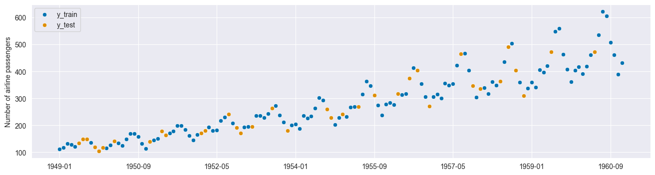
This leads to leakage:

The data you are using to train a machine learning algorithm happens to have the information you are trying to predict.

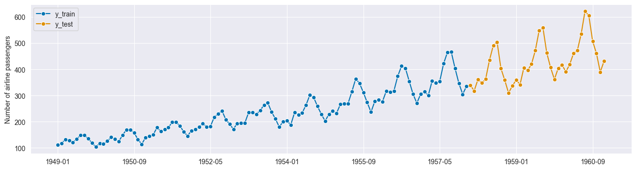
But train_test_split(y, shuffle=False) works, which is what temporal_train_test_split(y) does in aeon:

y_train, y_test = temporal_train_test_split(y)
plot_series(y_train, y_test, labels=["y_train", "y_test"]);

Pitfall 2: obscure data manipulations, brittle boilerplate code to apply regressors

It is common practice to apply supervised regressors after transforming the data for forecasting, through lagging - for example, in autoregressive reduction strategies.

Two important pitfalls appear right at the start:

• a lot of boilerplate code has to be written to transform the data to make it ready for fitting - this is highly error-prone

• there are a number of implicit hyperparameters here, such as window and lag size. If done without caution, these are not explicit or tracked in the experiment, which can lead to “p-value hacking”.

Below is an example of such boilerplate code to demonstrate this. The code is closely modelled on the R code used in the M4 competition:

# suppose we want to predict 3 years ahead
fh = np.arange(1, 37)

# slightly modified code from the M4 competition


def split_into_train_test(data, in_num, fh):
    """
    Splits the series into train and test sets.

    Each step takes multiple points as inputs
    :param data: an individual TS
    :param fh: number of out of sample points
    :param in_num: number of input points for the forecast
    :return:
    """
    train, test = data[:-fh], data[-(fh + in_num) :]
    x_train, y_train = train[:-1], np.roll(train, -in_num)[:-in_num]
    x_test, y_test = test[:-1], np.roll(test, -in_num)[:-in_num]
    #     x_test, y_test = train[-in_num:], np.roll(test, -in_num)[:-in_num]

    # reshape input to be [samples, time steps, features]
    # (N-NF samples, 1 time step, 1 feature)
    x_train = np.reshape(x_train, (-1, 1))
    x_test = np.reshape(x_test, (-1, 1))
    temp_test = np.roll(x_test, -1)
    temp_train = np.roll(x_train, -1)
    for _ in range(1, in_num):
        x_train = np.concatenate((x_train[:-1], temp_train[:-1]), 1)
        x_test = np.concatenate((x_test[:-1], temp_test[:-1]), 1)
        temp_test = np.roll(temp_test, -1)[:-1]
        temp_train = np.roll(temp_train, -1)[:-1]

    return x_train, y_train, x_test, y_test

# here we split the time index, rather than the actual values,
# to show how we split the windows
feature_window, target_window, _, _ = split_into_train_test(
    np.arange(len(y)), 10, len(fh)
)

To better understand the prior data transformation, we can look at how we can split the training series into windows. Here we show the generated windows expressed as integer indices:

feature_window[:5, :]

array([[ 0,  1,  2,  3,  4,  5,  6,  7,  8,  9],
       [ 1,  2,  3,  4,  5,  6,  7,  8,  9, 10],
       [ 2,  3,  4,  5,  6,  7,  8,  9, 10, 11],
       [ 3,  4,  5,  6,  7,  8,  9, 10, 11, 12],
       [ 4,  5,  6,  7,  8,  9, 10, 11, 12, 13]])

target_window[:5]

array([10, 11, 12, 13, 14])

# now we can split the actual values of the time series
x_train, y_train, x_test, y_test = split_into_train_test(y.values, 10, len(fh))
print(x_train.shape, y_train.shape)

(98, 10) (98,)

from sklearn.ensemble import RandomForestRegressor

model = RandomForestRegressor()
model.fit(x_train, y_train)

RandomForestRegressor()

In a Jupyter environment, please rerun this cell to show the HTML representation or trust the notebook.
On GitHub, the HTML representation is unable to render, please try loading this page with nbviewer.org.

To reiterate the potential pitfalls here:

The manual requires a lot of handwritten code which is often error-prone, not modular and not tuneable.

These steps involve a number of implicit hyperparameters:

• The way you slice the time series into windows (e.g. the window length);

• The way you generate forecasts (recursive strategy, direct strategy, other hybrid strategies).

Pitfall 3: Given a fitted regression algorithm, how can we generate forecasts?

The next important pitfall comes at the end:

If making predictions along the “manual route” for supervised regressors, the supervised regressor’s outputs have to be transformed back into forecasts. This is easily forgotten, and invites errors in forecasts and evaluation (see pitfall no.1) - especially, if one does not cleanly keep track of which data is known at what time, or how to invert the transformation made in fitting.

A naive user might now proceed like this:

print(x_test.shape, y_test.shape)

# add back time index to y_test
y_test = pd.Series(y_test, index=y.index[-len(fh) :])

(36, 10) (36,)

y_pred = model.predict(x_test)

from aeon.performance_metrics.forecasting import mean_absolute_percentage_error

mean_absolute_percentage_error(
    y_test, pd.Series(y_pred, index=y_test.index), symmetric=False
)

0.1036284801065993

So easy, so wrong … but what’s the problem here? It’s a bit subtle and not easy to spot:

We actually don’t make a multi-step-ahead forecast up to the 36th step ahead. Instead, we make 36 single-step-ahead forecasts always using the most recent data. But that’s a solution to a different learning task!

To fix this problem, we could write some code to do this recursively as in the M4 competition:

# slightly modified code from the M4 study
predictions = []
last_window = x_train[-1, :].reshape(1, -1)  # make it into 2d array

last_prediction = model.predict(last_window)[0]  # take value from array

for i in range(len(fh)):
    # append prediction
    predictions.append(last_prediction)

    # update last window using previously predicted value
    last_window[0] = np.roll(last_window[0], -1)
    last_window[0, (len(last_window[0]) - 1)] = last_prediction

    # predict next step ahead
    last_prediction = model.predict(last_window)[0]

y_pred_rec = pd.Series(predictions, index=y_test.index)

from aeon.performance_metrics.forecasting import mean_absolute_percentage_error

mean_absolute_percentage_error(
    y_test, pd.Series(y_pred_rec, index=y_test.index), symmetric=False
)

0.13520505245471068

To summarize the potential pitfalls here:

Obtaining regressor predictions and converting them back into forecasts is non-trivial and error-prone: * some boilerplate code needs to be written, which just as in pitfall no.2 introduces potential for problems; * It isn’t exactly obvious that this boilerplate code had to be written in the first place, creating a subtle failure point.

How does aeon help avoid the above pitfalls?

aeon mitigates the above pitfalls with:

• Its unified interface for forecasters - any strategy to produce forecasts is a forecaster. Through the unified interface, forecasters are directly compatible with deployment and evaluation workflows appropriate for forecasters;

• Its declarative specification interface that minimizes boilerplate code - it’s minimized to the bare necessities to tell aeon which forecaster you want to build.

Nevertheless, aeon aims to be flexible, and tries to avoid railroading the user into specific methodological choices.

from sklearn.neighbors import KNeighborsRegressor

from aeon.forecasting.compose import make_reduction

# declarative forecaster specification - just two lines!
regressor = KNeighborsRegressor(n_neighbors=1)
forecaster = make_reduction(regressor, window_length=15, strategy="recursive")

forecaster.fit(y_train)
y_pred = forecaster.predict(fh)

… and that’s it!

Note that there is no x_train or other boilerplate artefacts, since construction of the lagged features and other boilerplate code are taken care of by the forecaster internally.

For more details on the aeon composition interface, refer to Section 3 of the main forecasting tutorial.

---

Generated using nbsphinx. The Jupyter notebook can be found here.